Scientific Workflow with HSSM¶

Welcome to the scientific workflow tutorial. This tutorial starts with a basic experimental dataset and we will inch from a very simple HSSM model iteratively toward a model that captures many of the main patterns we can identify in our dataset.

Along the way we try to achieve the following balance:

1. Illustrate how HSSM can be used for real scientific workflows. HSSM helps us with model building, running the stats, and reporting results.
2. Allow this tutorial to be used as a first look into HSSM, shirking conceptually advanced features that are discused in the many dedicated tutorials you can find on the documentation

Colab Instructions¶

If you would like to run this tutorial on Google colab, please click this link.

Once you are in the colab:

1. Follow the installation instructions below (uncomment the respective code)
2. restart your runtime.

NOTE:

You may want to switch your runtime to have a GPU or TPU. To do so, go to Runtime > Change runtime type and select the desired hardware accelerator. Note that if you switch your runtime you have to follow the installation instructions again.

Install hssm¶

In [1]:

# If running this on Colab, please uncomment the next line
# !pip install hssm

# If running this on Colab, please uncomment the next line # !pip install hssm

Download tutorial data¶

In [2]:

# # Data Files
# !wget -P  data/carney_workshop_2025_data/ https://raw.githubusercontent.com/lnccbrown/HSSM/main/scientific_workflow_hssm/data/carney_workshop_2025_full.parquet
# !wget -P  data/carney_workshop_2025_data/ https://raw.githubusercontent.com/lnccbrown/HSSM/main/scientific_workflow_hssm/data/carney_workshop_2025_modeling.parquet
# !wget -P  data/carney_workshop_2025_data/ https://raw.githubusercontent.com/lnccbrown/HSSM/main/scientific_workflow_hssm/data/carney_workshop_2025_parameters.pkl

# # Presampled traces
# !wget -P  idata/basic_ddm/ https://raw.githubusercontent.com/lnccbrown/HSSM/main/scientific_workflow_hssm/idata/basic_ddm/traces.nc
# !wget -P  idata/ddm_hier/ https://raw.githubusercontent.com/lnccbrown/HSSM/main/scientific_workflow_hssm/idata/ddm_hier/traces.nc
# !wget -P  idata/angle_hier/ https://raw.githubusercontent.com/lnccbrown/HSSM/main/scientific_workflow_hssm/idata/angle_hier/traces.nc
# !wget -P  idata/angle_hier_v2/ https://raw.githubusercontent.com/lnccbrown/HSSM/main/scientific_workflow_hssm/idata/angle_hier_v2/traces.nc
# !wget -P  idata/angle_hier_v3/ https://raw.githubusercontent.com/lnccbrown/HSSM/main/scientific_workflow_hssm/idata/angle_hier_v3/traces.nc
# !wget -P  idata/angle_hier_v4/ https://raw.githubusercontent.com/lnccbrown/HSSM/main/scientific_workflow_hssm/idata/angle_hier_v4/traces.nc
# !wget -P  idata/angle_v5/ https://raw.githubusercontent.com/lnccbrown/HSSM/main/scientific_workflow_hssm/idata/angle_v5/traces.nc

# # Data Files # !wget -P data/carney_workshop_2025_data/ https://raw.githubusercontent.com/lnccbrown/HSSM/main/scientific_workflow_hssm/data/carney_workshop_2025_full.parquet # !wget -P data/carney_workshop_2025_data/ https://raw.githubusercontent.com/lnccbrown/HSSM/main/scientific_workflow_hssm/data/carney_workshop_2025_modeling.parquet # !wget -P data/carney_workshop_2025_data/ https://raw.githubusercontent.com/lnccbrown/HSSM/main/scientific_workflow_hssm/data/carney_workshop_2025_parameters.pkl # # Presampled traces # !wget -P idata/basic_ddm/ https://raw.githubusercontent.com/lnccbrown/HSSM/main/scientific_workflow_hssm/idata/basic_ddm/traces.nc # !wget -P idata/ddm_hier/ https://raw.githubusercontent.com/lnccbrown/HSSM/main/scientific_workflow_hssm/idata/ddm_hier/traces.nc # !wget -P idata/angle_hier/ https://raw.githubusercontent.com/lnccbrown/HSSM/main/scientific_workflow_hssm/idata/angle_hier/traces.nc # !wget -P idata/angle_hier_v2/ https://raw.githubusercontent.com/lnccbrown/HSSM/main/scientific_workflow_hssm/idata/angle_hier_v2/traces.nc # !wget -P idata/angle_hier_v3/ https://raw.githubusercontent.com/lnccbrown/HSSM/main/scientific_workflow_hssm/idata/angle_hier_v3/traces.nc # !wget -P idata/angle_hier_v4/ https://raw.githubusercontent.com/lnccbrown/HSSM/main/scientific_workflow_hssm/idata/angle_hier_v4/traces.nc # !wget -P idata/angle_v5/ https://raw.githubusercontent.com/lnccbrown/HSSM/main/scientific_workflow_hssm/idata/angle_v5/traces.nc

Start of Tutorial¶

Load modules¶

In [3]:

import warnings

import arviz as az
import numpy as np
import pandas as pd
from matplotlib import pyplot as plt

warnings.filterwarnings(
    "ignore",
    message="Numba will use object mode.*",
    category=UserWarning,
)
warnings.filterwarnings(
    "ignore",
    message="indexing past lexsort depth.*",
    category=pd.errors.PerformanceWarning,
)
warnings.filterwarnings(
    "ignore",
    message="Estimated shape parameter of Pareto.*",
    category=UserWarning,
)
warnings.filterwarnings(
    "ignore",
    message="There are not enough devices.*",
    category=UserWarning,
)
warnings.filterwarnings(
    "ignore",
    message="`init=.* is ignored by `nuts_sampler=.*",
    category=UserWarning,
)

import hssm

import warnings import arviz as az import numpy as np import pandas as pd from matplotlib import pyplot as plt warnings.filterwarnings( "ignore", message="Numba will use object mode.*", category=UserWarning, ) warnings.filterwarnings( "ignore", message="indexing past lexsort depth.*", category=pd.errors.PerformanceWarning, ) warnings.filterwarnings( "ignore", message="Estimated shape parameter of Pareto.*", category=UserWarning, ) warnings.filterwarnings( "ignore", message="There are not enough devices.*", category=UserWarning, ) warnings.filterwarnings( "ignore", message="`init=.* is ignored by `nuts_sampler=.*", category=UserWarning, ) import hssm

Load workshop data¶

In [4]:

def load_data(
    filename_base: str, folder: str = "data"
) -> tuple[pd.DataFrame, pd.DataFrame, dict]:
    """Load saved simulation data and parameters from files.

    Parameters
    ----------
    filename_base : str
        Base filename used when saving files
    folder : str, optional
        Folder containing saved files, by default "data"

    Returns
    -------
    tuple[pd.DataFrame, pd.DataFrame, dict]
        Contains:
        - DataFrame with modeling data
        - DataFrame with full data
        - Dict containing group and subject parameters
    """
    df_modeling = pd.read_parquet(f"{folder}/{filename_base}_modeling.parquet")
    return df_modeling

def load_data( filename_base: str, folder: str = "data" ) -> tuple[pd.DataFrame, pd.DataFrame, dict]: """Load saved simulation data and parameters from files. Parameters ---------- filename_base : str Base filename used when saving files folder : str, optional Folder containing saved files, by default "data" Returns ------- tuple[pd.DataFrame, pd.DataFrame, dict] Contains: - DataFrame with modeling data - DataFrame with full data - Dict containing group and subject parameters """ df_modeling = pd.read_parquet(f"{folder}/{filename_base}_modeling.parquet") return df_modeling

In [5]:

workshop_data = load_data(
    filename_base="carney_workshop_2025", folder="scientific_workflow_hssm/data/"
)

workshop_data = load_data( filename_base="carney_workshop_2025", folder="scientific_workflow_hssm/data/" )

Load Plotting Utilities¶

In [6]:

from mpl_toolkits.axes_grid1.inset_locator import inset_axes


def pretty_column_label(column: str | None) -> str:
    """Convert a data column name into a compact plot label."""
    if column is None:
        return "Condition"
    return column.replace("_", " ").title()


def plot_rt_by_choice(
    df: pd.DataFrame,
    categorical_column: str | None = None,
    colors: dict[str, str] | dict[int, str] | None = None,
    ax: plt.Axes | None = None,
):
    """Plot signed-RT histograms, optionally split by a categorical column."""
    if categorical_column is None:
        ax.hist(
            df["rt"] * df["response"],
            bins=np.linspace(-5, 5, 50),
            histtype="step",
            density=True,
            color="tab:blue",
        )
    else:
        for cond in df[categorical_column].unique():
            df_cond = df[df[categorical_column] == cond]
            ax.hist(
                df_cond["rt"] * df_cond["response"],
                bins=np.linspace(-5, 5, 50),
                label=str(cond),
                histtype="step",
                density=True,
                color=colors[cond],
            )
    ax.set_xlabel("RT * Choice")
    ax.set_ylabel("Density")
    return ax


def inset_bar_plot(
    df: pd.DataFrame,
    categorical_column: str,
    response_options: list[int],
    colors: dict[str, str] | dict[int, str] | None = None,
    ax: plt.Axes | None = None,
):
    """Draw an inset bar plot of choice proportions per response option."""
    axins = inset_axes(ax, width="42%", height="42%", loc="upper right", borderpad=0.35)
    bar_width = 0.45
    for j, resp in enumerate(response_options):
        for k, cond in enumerate(df[categorical_column].unique()):
            k_displace = -1 if k == 0 else 1
            df_cond = df[df[categorical_column] == cond]
            prop = df_cond[df_cond.response == resp].shape[0] / len(df_cond)
            axins.bar(
                (resp + ((bar_width / 2) * k_displace)),
                prop,
                width=bar_width,
                fill=False,
                edgecolor=colors[cond],
                label=f"Response {resp}",
            )
    axins.set_xticks(response_options)
    axins.set_ylim(0, 1)
    axins.set_yticks([0.0, 0.5, 1])
    axins.set_title("Choice prop.", fontsize=6)
    axins.tick_params(axis="both", which="major", labelsize=5, pad=1)
    axins.set_xlabel("")
    axins.set_ylabel("")
    return ax


def inset_bar_plot_vertical(
    df: pd.DataFrame,
    categorical_column: str,
    response_options: list[int],
    colors: dict[str, str] | dict[int, str] | None = None,
    ax: plt.Axes | None = None,
):
    """Draw an inset horizontal bar plot of mean RT per response option."""
    axins = inset_axes(ax, width="42%", height="42%", loc="upper right", borderpad=0.35)
    bar_width = 0.45
    for j, resp in enumerate(response_options):
        for k, cond in enumerate(df[categorical_column].unique()):
            k_displace = -1 if k == 0 else 1
            df_cond = df[df[categorical_column] == cond]
            rt_mean = (df_cond[df_cond.response == resp]).rt.mean()
            axins.barh(
                (resp + ((bar_width / 2) * k_displace)),
                rt_mean,
                height=bar_width,
                fill=False,
                edgecolor=colors[cond],
                label=f"Response {resp}",
            )

    axins.set_yticks(response_options)
    axins.set_xticks([0.0, 1.0, 2.0])
    axins.set_title("Mean RT", fontsize=6)
    axins.tick_params(axis="both", which="major", labelsize=5, pad=1)
    axins.set_xlabel("")
    axins.set_ylabel("")
    return ax


def plot_rt_hists(
    df: pd.DataFrame,
    by_participant: bool = True,
    split_by_column: str | None = None,
    inset_plot: str | None = "choice_proportion",
    cols: int = 5,
):
    """Plot RT histograms, optionally faceted by participant and category."""
    if split_by_column is not None:
        colors = {
            cond: color
            for cond, color in zip(
                df[split_by_column].unique(),
                ["tab:blue", "tab:orange", "tab:green", "tab:red", "tab:purple"],
            )
        }
    else:
        colors = None

    split_label = pretty_column_label(split_by_column)

    if by_participant:
        participants = df["participant_id"].unique()
        rows = (len(participants) + cols - 1) // cols
        fig, axes = plt.subplots(
            rows,
            cols,
            sharey=True,
            sharex=True,
            figsize=(cols * 2.7, rows * 2.15),
        )
        axes = axes.flatten()
        for i, pid in enumerate(participants):
            ax = axes[i]
            df_part = df[df["participant_id"] == pid]
            ax = plot_rt_by_choice(df_part, split_by_column, colors, ax)

            if split_by_column is not None and inset_plot == "choice_proportion":
                ax = inset_bar_plot(
                    df_part, split_by_column, df["response"].unique(), colors, ax
                )
            elif split_by_column is not None and inset_plot == "rt_mean":
                ax = inset_bar_plot_vertical(
                    df_part, split_by_column, df["response"].unique(), colors, ax
                )

        for j in range(i + 1, len(axes)):
            axes[j].set_visible(False)

        if split_by_column is not None:
            handles, labels = axes[0].get_legend_handles_labels()
            fig.legend(
                handles,
                labels,
                title=split_label,
                loc="upper left",
                bbox_to_anchor=(0.01, 0.98),
                fontsize="small",
            )

        fig.suptitle(f"RT, Split by {split_label} and Participant", y=0.995)
        fig.subplots_adjust(top=0.88, hspace=0.55, wspace=0.35)
        plt.show()
    else:
        fig, ax = plt.subplots(1, 1, figsize=(6, 4))
        ax = plot_rt_by_choice(df, split_by_column, colors, ax)

        if split_by_column is not None and inset_plot == "choice_proportion":
            ax = inset_bar_plot(
                df, split_by_column, df["response"].unique(), colors, ax
            )
        elif split_by_column is not None and inset_plot == "rt_mean":
            ax = inset_bar_plot_vertical(
                df, split_by_column, df["response"].unique(), colors, ax
            )

        if split_by_column is not None:
            ax.legend(title=split_label, loc="best", fontsize="small")
        fig.tight_layout()
        fig.suptitle(f"RT by Trial, Split by {split_label}", y=1.02)
        plt.show()


def plot_grouped_traces(traces, *, show_divergences: bool = True) -> None:
    """Plot every posterior variable in readable summary and participant groups."""
    summary_suffixes = ("_Intercept", "_mu", "_sigma")
    posterior_names = list(traces.posterior.data_vars)
    summary_names = [
        name for name in posterior_names if name.endswith(summary_suffixes)
    ]
    participant_names = [name for name in posterior_names if name not in summary_names]
    groups = (
        ("Population-level and group-scale parameters", summary_names),
        ("Participant-level effects", participant_names),
    )

    for title, var_names in groups:
        if not var_names:
            continue

        visuals = {
            "label": {"fontsize": 7, "labelpad": 2},
            "ticklabels": {"labelsize": 7},
        }
        if not show_divergences:
            visuals["divergence"] = False

        az.plot_trace_dist(
            traces,
            var_names=var_names,
            compact=True,
            visuals=visuals,
            figure_kwargs={
                "figsize": (13, max(6, 1.25 * len(var_names))),
                "layout": "constrained",
            },
        )
        figure = plt.gcf()
        figure.suptitle(title, fontsize=12)
        trace_axes = [axis for axis in figure.axes if axis.get_position().x0 > 0.5]
        for axis in trace_axes:
            axis.set_ylabel("")
            if axis is not trace_axes[-1]:
                axis.set_xlabel("")
        plt.show()

from mpl_toolkits.axes_grid1.inset_locator import inset_axes def pretty_column_label(column: str | None) -> str: """Convert a data column name into a compact plot label.""" if column is None: return "Condition" return column.replace("_", " ").title() def plot_rt_by_choice( df: pd.DataFrame, categorical_column: str | None = None, colors: dict[str, str] | dict[int, str] | None = None, ax: plt.Axes | None = None, ): """Plot signed-RT histograms, optionally split by a categorical column.""" if categorical_column is None: ax.hist( df["rt"] * df["response"], bins=np.linspace(-5, 5, 50), histtype="step", density=True, color="tab:blue", ) else: for cond in df[categorical_column].unique(): df_cond = df[df[categorical_column] == cond] ax.hist( df_cond["rt"] * df_cond["response"], bins=np.linspace(-5, 5, 50), label=str(cond), histtype="step", density=True, color=colors[cond], ) ax.set_xlabel("RT * Choice") ax.set_ylabel("Density") return ax def inset_bar_plot( df: pd.DataFrame, categorical_column: str, response_options: list[int], colors: dict[str, str] | dict[int, str] | None = None, ax: plt.Axes | None = None, ): """Draw an inset bar plot of choice proportions per response option.""" axins = inset_axes(ax, width="42%", height="42%", loc="upper right", borderpad=0.35) bar_width = 0.45 for j, resp in enumerate(response_options): for k, cond in enumerate(df[categorical_column].unique()): k_displace = -1 if k == 0 else 1 df_cond = df[df[categorical_column] == cond] prop = df_cond[df_cond.response == resp].shape[0] / len(df_cond) axins.bar( (resp + ((bar_width / 2) * k_displace)), prop, width=bar_width, fill=False, edgecolor=colors[cond], label=f"Response {resp}", ) axins.set_xticks(response_options) axins.set_ylim(0, 1) axins.set_yticks([0.0, 0.5, 1]) axins.set_title("Choice prop.", fontsize=6) axins.tick_params(axis="both", which="major", labelsize=5, pad=1) axins.set_xlabel("") axins.set_ylabel("") return ax def inset_bar_plot_vertical( df: pd.DataFrame, categorical_column: str, response_options: list[int], colors: dict[str, str] | dict[int, str] | None = None, ax: plt.Axes | None = None, ): """Draw an inset horizontal bar plot of mean RT per response option.""" axins = inset_axes(ax, width="42%", height="42%", loc="upper right", borderpad=0.35) bar_width = 0.45 for j, resp in enumerate(response_options): for k, cond in enumerate(df[categorical_column].unique()): k_displace = -1 if k == 0 else 1 df_cond = df[df[categorical_column] == cond] rt_mean = (df_cond[df_cond.response == resp]).rt.mean() axins.barh( (resp + ((bar_width / 2) * k_displace)), rt_mean, height=bar_width, fill=False, edgecolor=colors[cond], label=f"Response {resp}", ) axins.set_yticks(response_options) axins.set_xticks([0.0, 1.0, 2.0]) axins.set_title("Mean RT", fontsize=6) axins.tick_params(axis="both", which="major", labelsize=5, pad=1) axins.set_xlabel("") axins.set_ylabel("") return ax def plot_rt_hists( df: pd.DataFrame, by_participant: bool = True, split_by_column: str | None = None, inset_plot: str | None = "choice_proportion", cols: int = 5, ): """Plot RT histograms, optionally faceted by participant and category.""" if split_by_column is not None: colors = { cond: color for cond, color in zip( df[split_by_column].unique(), ["tab:blue", "tab:orange", "tab:green", "tab:red", "tab:purple"], ) } else: colors = None split_label = pretty_column_label(split_by_column) if by_participant: participants = df["participant_id"].unique() rows = (len(participants) + cols - 1) // cols fig, axes = plt.subplots( rows, cols, sharey=True, sharex=True, figsize=(cols * 2.7, rows * 2.15), ) axes = axes.flatten() for i, pid in enumerate(participants): ax = axes[i] df_part = df[df["participant_id"] == pid] ax = plot_rt_by_choice(df_part, split_by_column, colors, ax) if split_by_column is not None and inset_plot == "choice_proportion": ax = inset_bar_plot( df_part, split_by_column, df["response"].unique(), colors, ax ) elif split_by_column is not None and inset_plot == "rt_mean": ax = inset_bar_plot_vertical( df_part, split_by_column, df["response"].unique(), colors, ax ) for j in range(i + 1, len(axes)): axes[j].set_visible(False) if split_by_column is not None: handles, labels = axes[0].get_legend_handles_labels() fig.legend( handles, labels, title=split_label, loc="upper left", bbox_to_anchor=(0.01, 0.98), fontsize="small", ) fig.suptitle(f"RT, Split by {split_label} and Participant", y=0.995) fig.subplots_adjust(top=0.88, hspace=0.55, wspace=0.35) plt.show() else: fig, ax = plt.subplots(1, 1, figsize=(6, 4)) ax = plot_rt_by_choice(df, split_by_column, colors, ax) if split_by_column is not None and inset_plot == "choice_proportion": ax = inset_bar_plot( df, split_by_column, df["response"].unique(), colors, ax ) elif split_by_column is not None and inset_plot == "rt_mean": ax = inset_bar_plot_vertical( df, split_by_column, df["response"].unique(), colors, ax ) if split_by_column is not None: ax.legend(title=split_label, loc="best", fontsize="small") fig.tight_layout() fig.suptitle(f"RT by Trial, Split by {split_label}", y=1.02) plt.show() def plot_grouped_traces(traces, *, show_divergences: bool = True) -> None: """Plot every posterior variable in readable summary and participant groups.""" summary_suffixes = ("_Intercept", "_mu", "_sigma") posterior_names = list(traces.posterior.data_vars) summary_names = [ name for name in posterior_names if name.endswith(summary_suffixes) ] participant_names = [name for name in posterior_names if name not in summary_names] groups = ( ("Population-level and group-scale parameters", summary_names), ("Participant-level effects", participant_names), ) for title, var_names in groups: if not var_names: continue visuals = { "label": {"fontsize": 7, "labelpad": 2}, "ticklabels": {"labelsize": 7}, } if not show_divergences: visuals["divergence"] = False az.plot_trace_dist( traces, var_names=var_names, compact=True, visuals=visuals, figure_kwargs={ "figsize": (13, max(6, 1.25 * len(var_names))), "layout": "constrained", }, ) figure = plt.gcf() figure.suptitle(title, fontsize=12) trace_axes = [axis for axis in figure.axes if axis.get_position().x0 > 0.5] for axis in trace_axes: axis.set_ylabel("") if axis is not trace_axes[-1]: axis.set_xlabel("") plt.show()

Exploratory Data Analysis¶

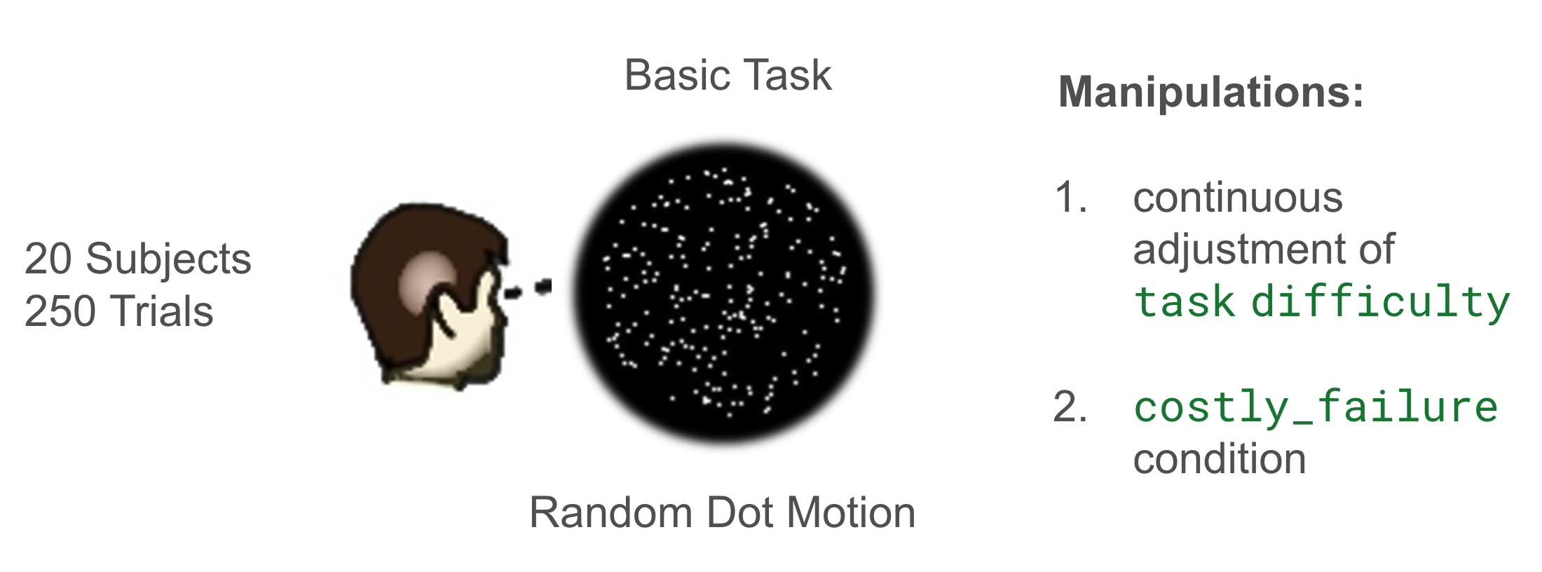
Now that we are done preparing the setup, let's get to the meat of it! The picture above gives us a bit of an idea, where the dataset that we are going to work with below comes from (alert: the backstory may or may not be real).

20 subjects, performed 250 trials each of a basic Random dot motion task. The task seemingly had two important manipulations.

1. A costly fail condition, in which subjects get punished for mistakes.
2. A trial by trail manipulation of difficulty (in the Random dot motion task, this refers to degree of coherence with which the dots move in a particular direction)

Let's take a look at the actual dataframe.

In [7]:

workshop_data

workshop_data

Out[7]:

	response	rt	participant_id	trial	costly_fail_condition	continuous_difficulty	response_l1
0	1	0.556439	0	1	1	-0.277337	0
1	1	0.741682	0	2	0	-0.810919	1
2	1	0.461832	0	3	0	-0.673330	1
3	1	0.626154	0	4	0	0.755445	1
4	1	0.651677	0	5	1	0.136755	1
...	...	...	...	...	...	...	...
4995	1	1.039342	19	246	0	-0.612223	-1
4996	1	1.587827	19	247	0	0.732396	1
4997	1	0.668594	19	248	1	-0.175321	1
4998	1	1.616471	19	249	0	-0.630447	1
4999	1	1.051329	19	250	1	0.511197	1

5000 rows × 7 columns

Adding a few columns¶

As part of prep work for plotting etc. we will add a few columns here. These will be motivated later (close your eyes :)).

In [8]:

# Binary version of difficulty
workshop_data["bin_difficulty"] = workshop_data["continuous_difficulty"].apply(
    lambda x: "high" if x > 0 else "low"
)

# I want a a ordinal variable that is composed of 5 quantile levels of difficulty
workshop_data["quantile_difficulty"] = pd.qcut(
    workshop_data["continuous_difficulty"], 3, labels=["-1", "0", "1"]
)

workshop_data["quantile_difficulty_binary"] = pd.qcut(
    workshop_data["continuous_difficulty"], 2, labels=["-1", "1"]
)

# Slightly
workshop_data["response_l1_plotting"] = workshop_data["response_l1"].apply(
    lambda x: str(-1) if x == -1 else str(1)
)

# Binary version of difficulty workshop_data["bin_difficulty"] = workshop_data["continuous_difficulty"].apply( lambda x: "high" if x > 0 else "low" ) # I want a a ordinal variable that is composed of 5 quantile levels of difficulty workshop_data["quantile_difficulty"] = pd.qcut( workshop_data["continuous_difficulty"], 3, labels=["-1", "0", "1"] ) workshop_data["quantile_difficulty_binary"] = pd.qcut( workshop_data["continuous_difficulty"], 2, labels=["-1", "1"] ) # Slightly workshop_data["response_l1_plotting"] = workshop_data["response_l1"].apply( lambda x: str(-1) if x == -1 else str(1) )

Most basic reaction time plot¶

In [9]:

plot_rt_hists(
    workshop_data, by_participant=False, split_by_column=None, inset_plot=None
)

plot_rt_hists( workshop_data, by_participant=False, split_by_column=None, inset_plot=None )

So far so good. Looking at the global reaction time pattern, it does seem commensurate with what we might expect out of basic Sequential Sampling Model (SSM). The basic DDM might be a good start here.

Basic Model: DDM¶

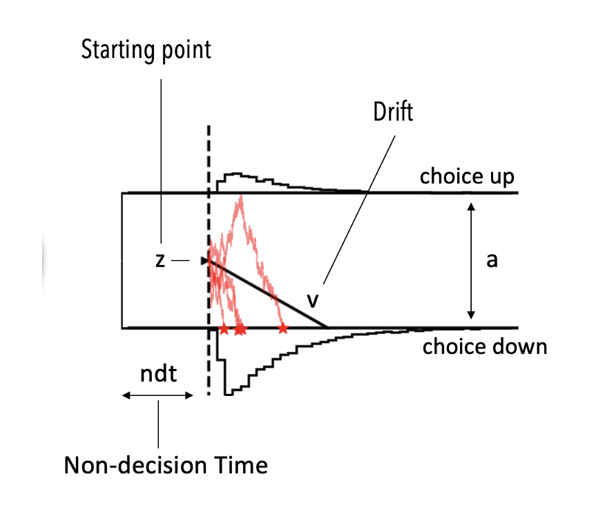
The picture above illustrates the basic Drift Diffusion Model. Note the parameters,

1. v the drift rate (how much evidence do I collect on average per unit of time)
2. a the boundary separation (how much evidence do I need to commit to a choice)
3. z how biased am I toward a particular choice a priori
4. ndt (we will simply call it t below), the delay between being exposed to a stimulus and starting the actual evidence accumulation process

In [10]:

BasicDDMModel = hssm.HSSM(
    data=workshop_data,
    model="ddm",
    loglik_kind="approx_differentiable",
    global_formula="y ~ 1",
    noncentered=False,
)

BasicDDMModel = hssm.HSSM( data=workshop_data, model="ddm", loglik_kind="approx_differentiable", global_formula="y ~ 1", noncentered=False, )

Model initialized successfully.

In [11]:

BasicDDMModel

BasicDDMModel

Out[11]:

Hierarchical Sequential Sampling Model
Model: ddm

Response variable: rt,response
Likelihood: approx_differentiable
Observations: 5000

Parameters:

v:
    Formula: v ~ 1
    Priors:
        v_Intercept ~ Normal(mu: 0.0, sigma: 0.25)
    Link: identity
    Explicit bounds: (-3.0, 3.0)

a:
    Formula: a ~ 1
    Priors:
        a_Intercept ~ Normal(mu: 1.4, sigma: 0.25)
    Link: identity
    Explicit bounds: (0.3, 2.5)

z:
    Formula: z ~ 1
    Priors:
        z_Intercept ~ Normal(mu: 0.5, sigma: 0.25)
    Link: identity
    Explicit bounds: (0.0, 1.0)

t:
    Formula: t ~ 1
    Priors:
        t_Intercept ~ Normal(mu: 1.0, sigma: 0.25)
    Link: identity
    Explicit bounds: (0.0, 2.0)


Lapse probability: 0.05
Lapse distribution: Uniform(lower: 0.0, upper: 20.0)

In [12]:

BasicDDMModel.graph()

BasicDDMModel.graph()

Out[12]:

In [13]:

try:
    # Load pre-computed traces
    BasicDDMModel.restore_traces(
        traces="scientific_workflow_hssm/idata/basic_ddm/traces.nc"
    )
except Exception:
    # Sample posterior
    basic_ddm_idata = BasicDDMModel.sample(
        chains=2,
        sampler="numpyro",
        tune=500,
        draws=500,
    )

    # Sample posterior predictive
    BasicDDMModel.sample_posterior_predictive(draws=200, safe_mode=True)

    # Save Model
    BasicDDMModel.save_model(
        model_name="basic_ddm",
        allow_absolute_base_path=True,
        base_path="scientific_workflow_hssm/idata/",
        save_idata_only=True,
    )

try: # Load pre-computed traces BasicDDMModel.restore_traces( traces="scientific_workflow_hssm/idata/basic_ddm/traces.nc" ) except Exception: # Sample posterior basic_ddm_idata = BasicDDMModel.sample( chains=2, sampler="numpyro", tune=500, draws=500, ) # Sample posterior predictive BasicDDMModel.sample_posterior_predictive(draws=200, safe_mode=True) # Save Model BasicDDMModel.save_model( model_name="basic_ddm", allow_absolute_base_path=True, base_path="scientific_workflow_hssm/idata/", save_idata_only=True, )

In [14]:

BasicDDMModel.traces

BasicDDMModel.traces

Out[14]:

<xarray.DataTree>
Group: /
│   Attributes:
│       inference_library:          numpyro
│       inference_library_version:  0.17.0
│       sampling_time:              95.06823
│       tuning_steps:               500
├── Group: /posterior
│       Dimensions:      (chain: 2, draw: 500)
│       Coordinates:
│         * chain        (chain) int64 16B 0 1
│         * draw         (draw) int64 4kB 0 1 2 3 4 5 6 ... 493 494 495 496 497 498 499
│       Data variables:
│           t_Intercept  (chain, draw) float64 8kB ...
│           z_Intercept  (chain, draw) float64 8kB ...
│           a_Intercept  (chain, draw) float64 8kB ...
│           v_Intercept  (chain, draw) float64 8kB ...
│       Attributes:
│           created_at:                  2025-07-11T17:29:22.668745+00:00
│           arviz_version:               0.21.0
│           inference_library:           numpyro
│           inference_library_version:   0.17.0
│           sampling_time:               95.06823
│           tuning_steps:                500
│           modeling_interface:          bambi
│           modeling_interface_version:  0.15.0
├── Group: /posterior_predictive
│       Dimensions:          (chain: 2, draw: 200, __obs__: 5000, rt,response_dim: 2)
│       Coordinates:
│         * chain            (chain) int64 16B 0 1
│         * draw             (draw) int64 2kB 0 1 2 3 4 5 6 ... 194 195 196 197 198 199
│         * __obs__          (__obs__) int64 40kB 0 1 2 3 4 ... 4995 4996 4997 4998 4999
│         * rt,response_dim  (rt,response_dim) int64 16B 0 1
│       Data variables:
│           rt,response      (chain, draw, __obs__, rt,response_dim) float64 32MB ...
│       Attributes:
│           modeling_interface:          bambi
│           modeling_interface_version:  0.15.0
├── Group: /log_likelihood
│       Dimensions:      (chain: 2, draw: 500, __obs__: 5000)
│       Coordinates:
│         * chain        (chain) int64 16B 0 1
│         * draw         (draw) int64 4kB 0 1 2 3 4 5 6 ... 493 494 495 496 497 498 499
│         * __obs__      (__obs__) int64 40kB 0 1 2 3 4 5 ... 4995 4996 4997 4998 4999
│       Data variables:
│           rt,response  (chain, draw, __obs__) float64 40MB ...
│       Attributes:
│           modeling_interface:          bambi
│           modeling_interface_version:  0.15.0
├── Group: /sample_stats
│       Dimensions:          (chain: 2, draw: 500)
│       Coordinates:
│         * chain            (chain) int64 16B 0 1
│         * draw             (draw) int64 4kB 0 1 2 3 4 5 6 ... 494 495 496 497 498 499
│       Data variables:
│           acceptance_rate  (chain, draw) float64 8kB ...
│           step_size        (chain, draw) float64 8kB ...
│           diverging        (chain, draw) bool 1kB ...
│           energy           (chain, draw) float64 8kB ...
│           n_steps          (chain, draw) int64 8kB ...
│           tree_depth       (chain, draw) int64 8kB ...
│           lp               (chain, draw) float64 8kB ...
│       Attributes:
│           created_at:                  2025-07-11T17:29:22.675898+00:00
│           arviz_version:               0.21.0
│           modeling_interface:          bambi
│           modeling_interface_version:  0.15.0
└── Group: /observed_data
        Dimensions:                  (__obs__: 5000, rt,response_extra_dim_0: 2)
        Coordinates:
          * __obs__                  (__obs__) int64 40kB 0 1 2 3 ... 4997 4998 4999
          * rt,response_extra_dim_0  (rt,response_extra_dim_0) int64 16B 0 1
        Data variables:
            rt,response              (__obs__, rt,response_extra_dim_0) float64 80kB ...
        Attributes:
            created_at:                  2025-07-11T17:29:22.676800+00:00
            arviz_version:               0.21.0
            inference_library:           numpyro
            inference_library_version:   0.17.0
            sampling_time:               95.06823
            tuning_steps:                500
            modeling_interface:          bambi
            modeling_interface_version:  0.15.0

xarray.DataTree

• /posterior(14)

  • Dimensions:
    • chain: 2
    • draw: 500
  • Coordinates: (2)
    • chain
      (chain)
      int64
      0 1

      array([0, 1])

    • draw
      (draw)
      int64
      0 1 2 3 4 5 ... 495 496 497 498 499

      array([  0,   1,   2, ..., 497, 498, 499], shape=(500,))

  • Data variables: (4)
    • t_Intercept
      (chain, draw)
      float64
      ...

      [1000 values with dtype=float64]

    • z_Intercept
      (chain, draw)
      float64
      ...

      [1000 values with dtype=float64]

    • a_Intercept
      (chain, draw)
      float64
      ...

      [1000 values with dtype=float64]

    • v_Intercept
      (chain, draw)
      float64
      ...

      [1000 values with dtype=float64]

  • Attributes: (8)

    created_at :

    2025-07-11T17:29:22.668745+00:00

    arviz_version :

    0.21.0

    inference_library :

    numpyro

    inference_library_version :

    0.17.0

    sampling_time :

    95.06823

    tuning_steps :

    500

    modeling_interface :

    bambi

    modeling_interface_version :

    0.15.0

  /posterior_predictive(7)

  • Dimensions:
    • chain: 2
    • draw: 200
    • __obs__: 5000
    • rt,response_dim: 2
  • Coordinates: (4)
    • chain
      (chain)
      int64
      0 1

      array([0, 1])

    • draw
      (draw)
      int64
      0 1 2 3 4 5 ... 195 196 197 198 199

      array([  0,   1,   2,   3,   4,   5,   6,   7,   8,   9,  10,  11,  12,  13,14,  15,  16,  17,  18,  19,  20,  21,  22,  23,  24,  25,  26,  27,28,  29,  30,  31,  32,  33,  34,  35,  36,  37,  38,  39,  40,  41,42,  43,  44,  45,  46,  47,  48,  49,  50,  51,  52,  53,  54,  55,56,  57,  58,  59,  60,  61,  62,  63,  64,  65,  66,  67,  68,  69,70,  71,  72,  73,  74,  75,  76,  77,  78,  79,  80,  81,  82,  83,84,  85,  86,  87,  88,  89,  90,  91,  92,  93,  94,  95,  96,  97,98,  99, 100, 101, 102, 103, 104, 105, 106, 107, 108, 109, 110, 111,112, 113, 114, 115, 116, 117, 118, 119, 120, 121, 122, 123, 124, 125,126, 127, 128, 129, 130, 131, 132, 133, 134, 135, 136, 137, 138, 139,140, 141, 142, 143, 144, 145, 146, 147, 148, 149, 150, 151, 152, 153,154, 155, 156, 157, 158, 159, 160, 161, 162, 163, 164, 165, 166, 167,168, 169, 170, 171, 172, 173, 174, 175, 176, 177, 178, 179, 180, 181,182, 183, 184, 185, 186, 187, 188, 189, 190, 191, 192, 193, 194, 195,196, 197, 198, 199])

    • __obs__
      (__obs__)
      int64
      0 1 2 3 4 ... 4996 4997 4998 4999

      array([   0,    1,    2, ..., 4997, 4998, 4999], shape=(5000,))

    • rt,response_dim
      (rt,response_dim)
      int64
      0 1

      array([0, 1])

  • Data variables: (1)
    • rt,response
      (chain, draw, __obs__, rt,response_dim)
      float64
      ...

      [4000000 values with dtype=float64]

  • Attributes: (2)

    modeling_interface :

    bambi

    modeling_interface_version :

    0.15.0

  /log_likelihood(6)

  • Dimensions:
    • chain: 2
    • draw: 500
    • __obs__: 5000
  • Coordinates: (3)
    • chain
      (chain)
      int64
      0 1

      array([0, 1])

    • draw
      (draw)
      int64
      0 1 2 3 4 5 ... 495 496 497 498 499

      array([  0,   1,   2, ..., 497, 498, 499], shape=(500,))

    • __obs__
      (__obs__)
      int64
      0 1 2 3 4 ... 4996 4997 4998 4999

      array([   0,    1,    2, ..., 4997, 4998, 4999], shape=(5000,))

  • Data variables: (1)
    • rt,response
      (chain, draw, __obs__)
      float64
      ...

      [5000000 values with dtype=float64]

  • Attributes: (2)

    modeling_interface :

    bambi

    modeling_interface_version :

    0.15.0

  /sample_stats(13)

  • Dimensions:
    • chain: 2
    • draw: 500
  • Coordinates: (2)
    • chain
      (chain)
      int64
      0 1

      array([0, 1])

    • draw
      (draw)
      int64
      0 1 2 3 4 5 ... 495 496 497 498 499

      array([  0,   1,   2, ..., 497, 498, 499], shape=(500,))

  • Data variables: (7)
    • acceptance_rate
      (chain, draw)
      float64
      ...

      [1000 values with dtype=float64]

    • step_size
      (chain, draw)
      float64
      ...

      [1000 values with dtype=float64]

    • diverging
      (chain, draw)
      bool
      ...

      [1000 values with dtype=bool]

    • energy
      (chain, draw)
      float64
      ...

      [1000 values with dtype=float64]

    • n_steps
      (chain, draw)
      int64
      ...

      [1000 values with dtype=int64]

    • tree_depth
      (chain, draw)
      int64
      ...

      [1000 values with dtype=int64]

    • lp
      (chain, draw)
      float64
      ...

      [1000 values with dtype=float64]

  • Attributes: (4)

    created_at :

    2025-07-11T17:29:22.675898+00:00

    arviz_version :

    0.21.0

    modeling_interface :

    bambi

    modeling_interface_version :

    0.15.0

  /observed_data(11)

  • Dimensions:
    • __obs__: 5000
    • rt,response_extra_dim_0: 2
  • Coordinates: (2)
    • __obs__
      (__obs__)
      int64
      0 1 2 3 4 ... 4996 4997 4998 4999

      array([   0,    1,    2, ..., 4997, 4998, 4999], shape=(5000,))

    • rt,response_extra_dim_0
      (rt,response_extra_dim_0)
      int64
      0 1

      array([0, 1])

  • Data variables: (1)
    • rt,response
      (__obs__, rt,response_extra_dim_0)
      float64
      ...

      [10000 values with dtype=float64]

  • Attributes: (8)

    created_at :

    2025-07-11T17:29:22.676800+00:00

    arviz_version :

    0.21.0

    inference_library :

    numpyro

    inference_library_version :

    0.17.0

    sampling_time :

    95.06823

    tuning_steps :

    500

    modeling_interface :

    bambi

    modeling_interface_version :

    0.15.0

• Attributes: (4)

  inference_library :

  numpyro

  inference_library_version :

  0.17.0

  sampling_time :

  95.06823

  tuning_steps :

  500

In [15]:

az.summary(BasicDDMModel.traces)

az.summary(BasicDDMModel.traces)

Out[15]:

	mean	sd	eti89_lb	eti89_ub	ess_bulk	ess_tail	r_hat	mcse_mean	mcse_sd
t_Intercept	0.3275	0.0054	0.32	0.34	576	609	1.00	0.00023	0.00016
z_Intercept	0.4659	0.0067	0.46	0.48	529	470	1.00	0.00029	0.00022
a_Intercept	1.0173	0.0088	1	1	582	550	1.00	0.00037	0.00025
v_Intercept	0.943	0.023	0.91	0.98	535	491	1.00	0.001	0.00074

In [16]:

az.plot_trace_dist(BasicDDMModel.traces)

az.plot_trace_dist(BasicDDMModel.traces)

Out[16]:

<arviz_plots.plot_collection.PlotCollection at 0x12e7ccbc0>

In [17]:

az.plot_forest(BasicDDMModel.traces)
plt.tight_layout()

az.plot_forest(BasicDDMModel.traces) plt.tight_layout()

In [18]:

az.plot_pair(
    BasicDDMModel.traces,
    marginal_kind="kde",
    visuals={"scatter": {"alpha": 0.25, "s": 8}},
)

az.plot_pair( BasicDDMModel.traces, marginal_kind="kde", visuals={"scatter": {"alpha": 0.25, "s": 8}}, )

Out[18]:

<arviz_plots.plot_matrix.PlotMatrix at 0x12e8cb710>

ArviZ 1.2 displays the off-diagonal pairwise relationships as posterior-draw scatter plots. The diagonal panels retain KDE marginals, so the figure shows both parameter dependence and marginal uncertainty.

In [19]:

ax = hssm.plotting.plot_model_cartoon(
    BasicDDMModel,
    n_samples=10,
    bins=20,
    plot_predictive_mean=True,
    plot_predictive_samples=False,
    # extra arguments for the underlying plot_model_cartoon() function
    n_trajectories=2,
);

ax = hssm.plotting.plot_model_cartoon( BasicDDMModel, n_samples=10, bins=20, plot_predictive_mean=True, plot_predictive_samples=False, # extra arguments for the underlying plot_model_cartoon() function n_trajectories=2, );

No posterior_predictive samples found. Generating posterior_predictive samples using the provided DataTree object and the original data. This will modify the provided DataTree object, or if not provided, the traces object stored inside the model.

In [20]:

ax = hssm.plotting.plot_quantile_probability(
    BasicDDMModel,
    cond="quantile_difficulty",
)
ax.set_ylim(0, 3);
# ax.set_xlim(-0.1, 1.1);

ax = hssm.plotting.plot_quantile_probability( BasicDDMModel, cond="quantile_difficulty", ) ax.set_ylim(0, 3); # ax.set_xlim(-0.1, 1.1);

In [21]:

ax = hssm.plotting.plot_quantile_probability(
    BasicDDMModel,
    cond="costly_fail_condition",
)
ax.set_ylim(0, 3);

ax = hssm.plotting.plot_quantile_probability( BasicDDMModel, cond="costly_fail_condition", ) ax.set_ylim(0, 3);

In [22]:

ax = hssm.plotting.plot_quantile_probability(
    BasicDDMModel,
    cond="response_l1_plotting",
)
ax.set_ylim(0, 3);

ax = hssm.plotting.plot_quantile_probability( BasicDDMModel, cond="response_l1_plotting", ) ax.set_ylim(0, 3);

In [23]:

# Posterior predictive
BasicDDMModel.plot_predictive(
    step=True, col="participant_id", col_wrap=5, bins=np.linspace(-5, 5, 50)
)

# Posterior predictive BasicDDMModel.plot_predictive( step=True, col="participant_id", col_wrap=5, bins=np.linspace(-5, 5, 50) )

Out[23]:

<seaborn.axisgrid.FacetGrid at 0x12f6c2030>

Taking stock¶

We can observe a few patterns here.

• First, cleary the reaction time distributions are not the same for every subject, we need to account for that.
• Second, I does seem like the tail of the reaction time distribution is more graceful in for our predictions than it is in the original subject data. (This was less clear when looking only at the global pattern...)

We will now adjust our model to tackle these patterns one by one. Let's begin by specializing our parameters by subject.

In Bayesian Inference we approach this by introducing a Hierarchy, we assume that subject level parameters derive from a common group distribution.

Inference then proceeds over the parameters of this group distribution, as well as the subject wise parameters.

Hierarchies serve as a form of regularization of our parameter estimates, the group distribution allows us to share information between the single subject parameters estimates.

You don't have to use a hierarchy, we could introduce a subject wise parameterization e.g. by simply treating participant_id as a categorical variable / collection of dummy variables without using any notion of a group distribution (and you are welcome to try this).

DDM Hierarchical¶

Moving on to our first hierarchical model. As a first step, we will use our global_formula argument to (1|participant_id), which is equivalent to 1 + (1|participant_id), (use 0 + (1|participant_id) is you explicitly don't want to create an intercept).

This will make all parameters of our model hierarchical.

In [24]:

DDMHierModel = hssm.HSSM(
    data=workshop_data,
    model="ddm",
    loglik_kind="approx_differentiable",
    global_formula="y ~ (1|participant_id)",  # New
    noncentered=False,
)

DDMHierModel = hssm.HSSM( data=workshop_data, model="ddm", loglik_kind="approx_differentiable", global_formula="y ~ (1|participant_id)", # New noncentered=False, )

Model initialized successfully.

In [25]:

try:
    # Load pre-computed traces
    DDMHierModel.restore_traces(
        traces="scientific_workflow_hssm/idata/ddm_hier/traces.nc"
    )
except Exception:
    # Sample posterior
    ddm_hier_idata = DDMHierModel.sample(
        chains=2,
        sampler="numpyro",
        tune=500,
        draws=500,
    )

    # Sample posterior predictive
    DDMHierModel.sample_posterior_predictive(draws=200, safe_mode=True)

    # Save Model
    DDMHierModel.save_model(
        model_name="ddm_hier",
        allow_absolute_base_path=True,
        base_path="scientific_workflow_hssm/idata/",
        save_idata_only=True,
    )

try: # Load pre-computed traces DDMHierModel.restore_traces( traces="scientific_workflow_hssm/idata/ddm_hier/traces.nc" ) except Exception: # Sample posterior ddm_hier_idata = DDMHierModel.sample( chains=2, sampler="numpyro", tune=500, draws=500, ) # Sample posterior predictive DDMHierModel.sample_posterior_predictive(draws=200, safe_mode=True) # Save Model DDMHierModel.save_model( model_name="ddm_hier", allow_absolute_base_path=True, base_path="scientific_workflow_hssm/idata/", save_idata_only=True, )

In [26]:

DDMHierModel.graph()

DDMHierModel.graph()

Out[26]:

In [27]:

plot_grouped_traces(DDMHierModel.traces)

plot_grouped_traces(DDMHierModel.traces)

In [28]:

ax = hssm.plotting.plot_model_cartoon(
    DDMHierModel,
    col="participant_id",
    col_wrap=5,
    n_samples=100,
    bin_size=0.2,
    plot_predictive_mean=True,
    # color_pp_mean = "red",
    # color_pp = "black",
    plot_predictive_samples=False,
    # extra arguments for the underlying plot_model_cartoon() function
    n_trajectories=2,
);

ax = hssm.plotting.plot_model_cartoon( DDMHierModel, col="participant_id", col_wrap=5, n_samples=100, bin_size=0.2, plot_predictive_mean=True, # color_pp_mean = "red", # color_pp = "black", plot_predictive_samples=False, # extra arguments for the underlying plot_model_cartoon() function n_trajectories=2, );

No posterior_predictive samples found. Generating posterior_predictive samples using the provided DataTree object and the original data. This will modify the provided DataTree object, or if not provided, the traces object stored inside the model.

Comparing Parameter Loadings¶

In [29]:

az.summary(
    DDMHierModel.traces, filter_vars="like", var_names=["~participant_id"]
).sort_index()

az.summary( DDMHierModel.traces, filter_vars="like", var_names=["~participant_id"] ).sort_index()

Out[29]:

	mean	sd	eti89_lb	eti89_ub	ess_bulk	ess_tail	r_hat	mcse_mean	mcse_sd
a_Intercept	1.041	0.019	1	1.1	310	381	1.01	0.0011	0.00076
t_Intercept	0.375	0.021	0.34	0.41	89	138	1.01	0.0023	0.0019
v_Intercept	0.95	0.11	0.76	1.1	121	144	1.01	0.01	0.0071
z_Intercept	0.455	0.016	0.43	0.48	189	226	1.01	0.0012	0.00084

In [30]:

az.summary(BasicDDMModel.traces).sort_index()

az.summary(BasicDDMModel.traces).sort_index()

Out[30]:

	mean	sd	eti89_lb	eti89_ub	ess_bulk	ess_tail	r_hat	mcse_mean	mcse_sd
a_Intercept	1.0173	0.0088	1	1	582	550	1.00	0.00037	0.00025
t_Intercept	0.3275	0.0054	0.32	0.34	576	609	1.00	0.00023	0.00016
v_Intercept	0.943	0.023	0.91	0.98	535	491	1.00	0.001	0.00074
z_Intercept	0.4659	0.0067	0.46	0.48	529	470	1.00	0.00029	0.00022

The mean parameters of our models are de facto quite similar. Allowing subject wise variation however dramatically improved our fit to the data!

Quantitative Model Comparison¶

In [31]:

az.compare({"DDM": BasicDDMModel.traces, "DDM Hierarchical": DDMHierModel.traces})

az.compare({"DDM": BasicDDMModel.traces, "DDM Hierarchical": DDMHierModel.traces})

Out[31]:

	rank	elpd_diff	dse	p_worse	diag_diff	diag_elpd	p	elpd	se	weight
DDM Hierarchical	0	0.0	0.0	NaN		1 k̂ > 0.67	74.5	-5000.0	76.0	1.0
DDM	1	-690.0	33.0	1.0			4.8	-5600.0	75.0	0.0

Comparing predictions¶

In [32]:

# Posterior predictive
DDMHierModel.plot_predictive(step=True, col_wrap=5, bins=np.linspace(-5, 5, 50));

# Posterior predictive DDMHierModel.plot_predictive(step=True, col_wrap=5, bins=np.linspace(-5, 5, 50));

In [33]:

# Posterior predictive
BasicDDMModel.plot_predictive(step=True, col_wrap=5, bins=np.linspace(-5, 5, 50));

# Posterior predictive BasicDDMModel.plot_predictive(step=True, col_wrap=5, bins=np.linspace(-5, 5, 50));

In [34]:

# Posterior predictive
DDMHierModel.plot_predictive(
    step=True, col="participant_id", col_wrap=5, bins=np.linspace(-5, 5, 50)
)

# Posterior predictive DDMHierModel.plot_predictive( step=True, col="participant_id", col_wrap=5, bins=np.linspace(-5, 5, 50) )

Out[34]:

<seaborn.axisgrid.FacetGrid at 0x12fdc4e00>

Taking Stock¶

Let's take stock again of any obvious pontential for improving our model here. We are now capturing the data much better subject by subject, however looking closely,

it seems like the tail behavior of the observed and the predicted data is somewhat different, for a few subjects.

The particularly suspicious subjest, are:

• participant_id = 1
• participant_id = 14
• participant_id = 15
• participant_id = 17

It seems that for these (and there are others) participants, the model predicted data has a wider tail than what we actually observe in our dataset.

This will motivate a change in the Sequential Sampling Model that we apply.

Angle Model Hierarchical¶

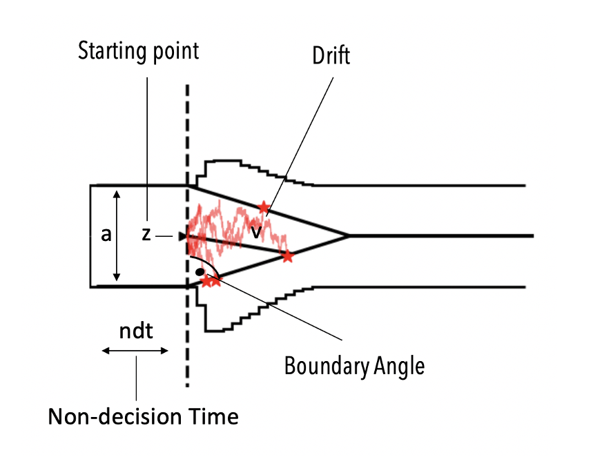
Given what we concluded about the tail behavior of the observed RTs, we will adjust our SSM, to allow for linear collapsing bounds. HSSM ships with a such a model, and we can apply it to our data simple by changing the model argument. The corresponding model is called angle model in our lingo, and is illustrated below conceptually.

In [35]:

AngleHierModel = hssm.HSSM(
    data=workshop_data,
    model="angle",
    loglik_kind="approx_differentiable",
    global_formula="y ~ (1|participant_id)",
    noncentered=False,
)

AngleHierModel = hssm.HSSM( data=workshop_data, model="angle", loglik_kind="approx_differentiable", global_formula="y ~ (1|participant_id)", noncentered=False, )

Model initialized successfully.

In [36]:

AngleHierModel.graph()

AngleHierModel.graph()

Out[36]:

In [37]:

try:
    # Load pre-computed traces
    AngleHierModel.restore_traces(
        traces="scientific_workflow_hssm/idata/angle_hier/traces.nc"
    )
except Exception:
    # Sample posterior
    angle_hier_idata = AngleHierModel.sample(
        chains=2,
        sampler="numpyro",
        tune=500,
        draws=500,
    )

    # Sample posterior predictive
    AngleHierModel.sample_posterior_predictive(draws=200, safe_mode=True)

    # Save Model
    AngleHierModel.save_model(
        model_name="angle_hier",
        allow_absolute_base_path=True,
        base_path="scientific_workflow_hssm/idata/",
        save_idata_only=True,
    )

try: # Load pre-computed traces AngleHierModel.restore_traces( traces="scientific_workflow_hssm/idata/angle_hier/traces.nc" ) except Exception: # Sample posterior angle_hier_idata = AngleHierModel.sample( chains=2, sampler="numpyro", tune=500, draws=500, ) # Sample posterior predictive AngleHierModel.sample_posterior_predictive(draws=200, safe_mode=True) # Save Model AngleHierModel.save_model( model_name="angle_hier", allow_absolute_base_path=True, base_path="scientific_workflow_hssm/idata/", save_idata_only=True, )

In [38]:

ax = hssm.plotting.plot_model_cartoon(
    AngleHierModel,
    col="participant_id",
    col_wrap=5,
    n_samples=10,
    bin_size=0.2,
    plot_predictive_mean=True,
    plot_predictive_samples=False,
    # extra arguments for the underlying plot_model_cartoon() function
    n_trajectories=2,
);

ax = hssm.plotting.plot_model_cartoon( AngleHierModel, col="participant_id", col_wrap=5, n_samples=10, bin_size=0.2, plot_predictive_mean=True, plot_predictive_samples=False, # extra arguments for the underlying plot_model_cartoon() function n_trajectories=2, );

No posterior_predictive samples found. Generating posterior_predictive samples using the provided DataTree object and the original data. This will modify the provided DataTree object, or if not provided, the traces object stored inside the model.

We can up it one notch and include the parameter uncertainty in the model_cartoon_plot(). This helps us assess how certain we are about the setting of the boundary collapse here. Let's see what that looks like!

In [39]:

ax = hssm.plotting.plot_model_cartoon(
    AngleHierModel,
    col="participant_id",
    col_wrap=5,
    n_samples=50,
    bin_size=0.2,
    plot_predictive_mean=True,
    plot_predictive_samples=True,
    # extra arguments for the underlying plot_model_cartoon() function
    n_trajectories=2,
);

ax = hssm.plotting.plot_model_cartoon( AngleHierModel, col="participant_id", col_wrap=5, n_samples=50, bin_size=0.2, plot_predictive_mean=True, plot_predictive_samples=True, # extra arguments for the underlying plot_model_cartoon() function n_trajectories=2, );

No posterior_predictive samples found. Generating posterior_predictive samples using the provided DataTree object and the original data. This will modify the provided DataTree object, or if not provided, the traces object stored inside the model.

Angle (theta) parameter Bayesian t-test¶

In [40]:

pc = az.plot_dist(AngleHierModel.traces, var_names=["theta_Intercept"], kind="hist")
az.add_lines(
    pc,
    values={"theta_Intercept": 0},
    orientation="vertical",
    visuals={"ref_line": dict(color="red", linestyle="--")},
)

pc = az.plot_dist(AngleHierModel.traces, var_names=["theta_Intercept"], kind="hist") az.add_lines( pc, values={"theta_Intercept": 0}, orientation="vertical", visuals={"ref_line": dict(color="red", linestyle="--")}, )

Out[40]:

<arviz_plots.plot_collection.PlotCollection at 0x13221fad0>

In [41]:

# Posterior predictive
AngleHierModel.plot_predictive(step=True, col_wrap=5, bins=np.linspace(-5, 5, 50))

# Posterior predictive AngleHierModel.plot_predictive(step=True, col_wrap=5, bins=np.linspace(-5, 5, 50))

Out[41]:

<Axes: title={'center': 'Posterior Predictive Distribution'}, xlabel='Response Time', ylabel='Density'>

In [42]:

# Posterior predictive
AngleHierModel.plot_predictive(
    step=True, col="participant_id", col_wrap=5, bins=np.linspace(-5, 5, 50)
)

# Posterior predictive AngleHierModel.plot_predictive( step=True, col="participant_id", col_wrap=5, bins=np.linspace(-5, 5, 50) )

Out[42]:

<seaborn.axisgrid.FacetGrid at 0x149f48f50>

Visually it seems like we did improve the fit (even though the difference in visual improvement is much less than what we had witnessed introducing the hierarchy in the first place).

Let us corroborate the visual intuition via formal model comparison.

Quantitative Model Comparison¶

In [43]:

az.compare(
    {
        "DDM": BasicDDMModel.traces,
        "DDM Hierarchical": DDMHierModel.traces,
        "Angle Hierarchical": AngleHierModel.traces,
    }
)

az.compare( { "DDM": BasicDDMModel.traces, "DDM Hierarchical": DDMHierModel.traces, "Angle Hierarchical": AngleHierModel.traces, } )

Out[43]:

	rank	elpd_diff	dse	p_worse	diag_diff	diag_elpd	p	elpd	se	weight
Angle Hierarchical	0	0.0	0.0	NaN			78.3	-4700.0	73.0	1.0
DDM Hierarchical	1	-220.0	16.0	1.0		1 k̂ > 0.67	74.5	-5000.0	76.0	0.0
DDM	2	-910.0	36.0	1.0			4.8	-5600.0	75.0	0.0

Good, introducing the angle model seemed to have helped us quite a bit, even though, as intuited by the simple visual inspection, the improvement in elpd_loo is not as the improvement in going from a simple model toward a hierarchical model (even though the actual SSM was misspecified).

So what next? On the surface, it looks like we have a model that fits our data quite well.

Let's take another look at our data to identify more patterns that we may not capture with out current efforts.

Further EDA¶

Maybe it is time to look more directly at the effects of our experiment manipulations.

Below are a few graphs to understand what might be happening.

In [44]:

# Posterior predictive
AngleHierModel.plot_predictive(
    step=True, col="costly_fail_condition", bins=np.linspace(-5, 5, 50)
)
plt.tight_layout()

# Posterior predictive AngleHierModel.plot_predictive( step=True, col="costly_fail_condition", bins=np.linspace(-5, 5, 50) ) plt.tight_layout()

In [45]:

ax = hssm.plotting.plot_quantile_probability(
    AngleHierModel,
    cond="costly_fail_condition",
)
ax.set_ylim(0, 3);

ax = hssm.plotting.plot_quantile_probability( AngleHierModel, cond="costly_fail_condition", ) ax.set_ylim(0, 3);

In [46]:

plot_rt_hists(
    workshop_data,
    by_participant=True,
    split_by_column="costly_fail_condition",
    inset_plot="choice_proportion",
)

plot_rt_hists( workshop_data, by_participant=True, split_by_column="costly_fail_condition", inset_plot="choice_proportion", )

In [47]:

plot_rt_hists(
    workshop_data,
    by_participant=True,
    split_by_column="costly_fail_condition",
    inset_plot="rt_mean",
)

plot_rt_hists( workshop_data, by_participant=True, split_by_column="costly_fail_condition", inset_plot="rt_mean", )

We can identify two patterns.

1. On average in the costly_fail_condition participants seem to make slightly fewer mistakes
2. On average in the costly_fail_condition participants seem to take a little longer for their choices!

This meshes with how we expect the incentives to act. Participants should be slightly more cautious to get it right, if mistakes are costly!

In the contect of SSMs, this is usually mapped on to the decision threshold (parameter a), so maybe we should try to incorporate the costly_fail_condition in the regression function for that parameter in our model.

Addressing costly fail condition¶

To include parameter specific regressions, we can rely on the include argument in HSSM. Let's illustrate this.

In [48]:

AngleHierModelV2 = hssm.HSSM(
    data=workshop_data,
    model="angle",
    loglik_kind="approx_differentiable",
    global_formula="y ~ (1|participant_id)",
    include=[
        {"name": "a", "formula": "a ~ (1 + C(costly_fail_condition)|participant_id)"}
    ],
    noncentered=False,
)

AngleHierModelV2 = hssm.HSSM( data=workshop_data, model="angle", loglik_kind="approx_differentiable", global_formula="y ~ (1|participant_id)", include=[ {"name": "a", "formula": "a ~ (1 + C(costly_fail_condition)|participant_id)"} ], noncentered=False, )

Model initialized successfully.

In [49]:

AngleHierModelV2.graph()

AngleHierModelV2.graph()

Out[49]:

In [50]:

try:
    # Load pre-computed traces
    AngleHierModelV2.restore_traces(
        traces="scientific_workflow_hssm/idata/angle_hier_v2/traces.nc"
    )
except Exception:
    # Sample posterior
    angle_hier_idata = AngleHierModelV2.sample(
        chains=2,
        sampler="numpyro",
        tune=500,
        draws=500,
    )

    # Sample posterior predictive
    AngleHierModelV2.sample_posterior_predictive(draws=200, safe_mode=True)

    # Save Model
    AngleHierModelV2.save_model(
        model_name="angle_hier_v2",
        allow_absolute_base_path=True,
        base_path="scientific_workflow_hssm/idata/",
        save_idata_only=True,
    )

try: # Load pre-computed traces AngleHierModelV2.restore_traces( traces="scientific_workflow_hssm/idata/angle_hier_v2/traces.nc" ) except Exception: # Sample posterior angle_hier_idata = AngleHierModelV2.sample( chains=2, sampler="numpyro", tune=500, draws=500, ) # Sample posterior predictive AngleHierModelV2.sample_posterior_predictive(draws=200, safe_mode=True) # Save Model AngleHierModelV2.save_model( model_name="angle_hier_v2", allow_absolute_base_path=True, base_path="scientific_workflow_hssm/idata/", save_idata_only=True, )

In [51]:

plot_grouped_traces(AngleHierModelV2.traces)

plot_grouped_traces(AngleHierModelV2.traces)

In [52]:

pc = az.plot_dist(
    AngleHierModelV2.traces,
    var_names=["a_C(costly_fail_condition)|participant_id_mu"],
    kind="hist",
)
az.add_lines(
    pc,
    values={"a_C(costly_fail_condition)|participant_id_mu": 0},
    orientation="vertical",
    visuals={"ref_line": dict(color="red", linestyle="--")},
)

pc = az.plot_dist( AngleHierModelV2.traces, var_names=["a_C(costly_fail_condition)|participant_id_mu"], kind="hist", ) az.add_lines( pc, values={"a_C(costly_fail_condition)|participant_id_mu": 0}, orientation="vertical", visuals={"ref_line": dict(color="red", linestyle="--")}, )

Out[52]:

<arviz_plots.plot_collection.PlotCollection at 0x1304bcf80>

In [53]:

# Posterior predictive
AngleHierModelV2.plot_predictive(
    step=True,
    # row = 'participant_id',
    col="costly_fail_condition",
    bins=np.linspace(-5, 5, 50),
)
plt.tight_layout()
plt.show()

# Posterior predictive AngleHierModelV2.plot_predictive( step=True, # row = 'participant_id', col="costly_fail_condition", bins=np.linspace(-5, 5, 50), ) plt.tight_layout() plt.show()

In [54]:

ax = hssm.plotting.plot_quantile_probability(
    AngleHierModelV2,
    cond="costly_fail_condition",
)
ax.set_ylim(0, 3);

ax = hssm.plotting.plot_quantile_probability( AngleHierModelV2, cond="costly_fail_condition", ) ax.set_ylim(0, 3);

Quite an improvement! Let's see what our quantitative model comparison metrics say.

Quantitative Model Comparison¶

In [55]:

az.compare(
    {
        "DDM": BasicDDMModel.traces,
        "DDM Hierarchical": DDMHierModel.traces,
        "Angle Hierarchical": AngleHierModel.traces,
        "Angle Hierarchical Cost": AngleHierModelV2.traces,
    }
)

az.compare( { "DDM": BasicDDMModel.traces, "DDM Hierarchical": DDMHierModel.traces, "Angle Hierarchical": AngleHierModel.traces, "Angle Hierarchical Cost": AngleHierModelV2.traces, } )

Out[55]:

	rank	elpd_diff	dse	p_worse	diag_diff	diag_elpd	p	elpd	se	weight
Angle Hierarchical Cost	0	0.0	0.0	NaN			87.5	-4500.0	71.0	1.0
Angle Hierarchical	1	-270.0	20.0	1.0			78.3	-4700.0	73.0	0.0
DDM Hierarchical	2	-480.0	25.0	1.0		1 k̂ > 0.67	74.5	-5000.0	76.0	0.0
DDM	3	-1170.0	41.0	1.0			4.8	-5600.0	75.0	0.0

Good, we now incorporated the costly_fail_condition in a conceptually coherent manner.

Let's take a look at difficulty next.

In [56]:

ax = hssm.plotting.plot_quantile_probability(
    AngleHierModelV2,
    cond="quantile_difficulty_binary",
)
ax.set_ylim(0, 3);

ax = hssm.plotting.plot_quantile_probability( AngleHierModelV2, cond="quantile_difficulty_binary", ) ax.set_ylim(0, 3);

In [57]:

plot_rt_hists(
    workshop_data,
    by_participant=True,
    split_by_column="quantile_difficulty_binary",
    inset_plot="rt_mean",
)

plot_rt_hists( workshop_data, by_participant=True, split_by_column="quantile_difficulty_binary", inset_plot="rt_mean", )

In [58]:

plot_rt_hists(
    workshop_data,
    by_participant=True,
    split_by_column="quantile_difficulty_binary",
    inset_plot="choice_proportion",
)

plot_rt_hists( workshop_data, by_participant=True, split_by_column="quantile_difficulty_binary", inset_plot="choice_proportion", )

We see a similar pattern. Difficulty affects choice probability, however the effect on RT is less clear.

What parameter should difficulty map onto? Usually it maps onto the rate of evidence accumulation, which is the drift (v) parameter most SSMs.

We will move ahead and try this. To add specialized regression for v we can add another parameter dictionary to the list we pass to include.

Addressing difficulty¶

In [59]:

AngleHierModelV3 = hssm.HSSM(
    data=workshop_data,
    model="angle",
    loglik_kind="approx_differentiable",
    global_formula="y ~ (1|participant_id)",
    include=[
        {"name": "a", "formula": "a ~ (1 + C(costly_fail_condition)|participant_id)"},
        {"name": "v", "formula": "v ~ (1 + continuous_difficulty|participant_id)"},
    ],
    noncentered=False,
)

AngleHierModelV3 = hssm.HSSM( data=workshop_data, model="angle", loglik_kind="approx_differentiable", global_formula="y ~ (1|participant_id)", include=[ {"name": "a", "formula": "a ~ (1 + C(costly_fail_condition)|participant_id)"}, {"name": "v", "formula": "v ~ (1 + continuous_difficulty|participant_id)"}, ], noncentered=False, )

Model initialized successfully.

In [60]:

AngleHierModelV3.graph()

AngleHierModelV3.graph()

Out[60]:

In [61]:

try:
    # Load pre-computed traces
    AngleHierModelV3.restore_traces(
        traces="scientific_workflow_hssm/idata/angle_hier_v3/traces.nc"
    )
except Exception:
    # Sample posterior
    angle_hier_idata = AngleHierModelV3.sample(
        chains=2,
        sampler="numpyro",
        tune=500,
        draws=500,
    )

    # Sample posterior predictive
    AngleHierModelV3.sample_posterior_predictive(draws=200, safe_mode=True)

    # Save Model
    AngleHierModelV3.save_model(
        model_name="angle_hier_v3",
        allow_absolute_base_path=True,
        base_path="scientific_workflow_hssm/idata/",
        save_idata_only=True,
    )

try: # Load pre-computed traces AngleHierModelV3.restore_traces( traces="scientific_workflow_hssm/idata/angle_hier_v3/traces.nc" ) except Exception: # Sample posterior angle_hier_idata = AngleHierModelV3.sample( chains=2, sampler="numpyro", tune=500, draws=500, ) # Sample posterior predictive AngleHierModelV3.sample_posterior_predictive(draws=200, safe_mode=True) # Save Model AngleHierModelV3.save_model( model_name="angle_hier_v3", allow_absolute_base_path=True, base_path="scientific_workflow_hssm/idata/", save_idata_only=True, )

In [62]:

pc = az.plot_dist(
    AngleHierModelV3.traces,
    var_names=["v_continuous_difficulty|participant_id_mu"],
    kind="hist",
)
az.add_lines(
    pc,
    values={"v_continuous_difficulty|participant_id_mu": 0},
    orientation="vertical",
    visuals={"ref_line": dict(color="red", linestyle="--")},
)

pc = az.plot_dist( AngleHierModelV3.traces, var_names=["v_continuous_difficulty|participant_id_mu"], kind="hist", ) az.add_lines( pc, values={"v_continuous_difficulty|participant_id_mu": 0}, orientation="vertical", visuals={"ref_line": dict(color="red", linestyle="--")}, )

Out[62]:

<arviz_plots.plot_collection.PlotCollection at 0x12f7cef30>

Looks like the effect on v is small (to the trained eye :)), but it is significant! Let's check if we can account for the data pattern we missed previously.

In [63]:

ax = hssm.plotting.plot_quantile_probability(
    AngleHierModelV3,
    cond="quantile_difficulty_binary",
)
ax.set_ylim(0, 3);

ax = hssm.plotting.plot_quantile_probability( AngleHierModelV3, cond="quantile_difficulty_binary", ) ax.set_ylim(0, 3);

In [64]:

# Posterior predictive
AngleHierModelV3.plot_predictive(
    step=True, col="quantile_difficulty_binary", bins=np.linspace(-5, 5, 50)
)
plt.tight_layout()

# Posterior predictive AngleHierModelV3.plot_predictive( step=True, col="quantile_difficulty_binary", bins=np.linspace(-5, 5, 50) ) plt.tight_layout()

Success! This looks much better.

Quantitative Model Comparison¶

In [65]:

az.compare(
    {
        "DDM": BasicDDMModel.traces,
        "DDM Hierarchical": DDMHierModel.traces,
        "Angle Hierarchical": AngleHierModel.traces,
        "Angle Hierarchical Cost": AngleHierModelV2.traces,
        "Angle Hierarchical Cost/Diff": AngleHierModelV3.traces,
    }
)

az.compare( { "DDM": BasicDDMModel.traces, "DDM Hierarchical": DDMHierModel.traces, "Angle Hierarchical": AngleHierModel.traces, "Angle Hierarchical Cost": AngleHierModelV2.traces, "Angle Hierarchical Cost/Diff": AngleHierModelV3.traces, } )

Out[65]:

	rank	elpd_diff	dse	p_worse	diag_diff	diag_elpd	p	elpd	se	weight
Angle Hierarchical Cost/Diff	0	0.0	0.0	NaN		84 k̂ > 0.67	69.2	-4400.0	71.0	0.99
Angle Hierarchical Cost	1	-40.0	9.6	1.0			87.5	-4500.0	71.0	0.01
Angle Hierarchical	2	-310.0	23.0	1.0			78.3	-4700.0	73.0	0.00
DDM Hierarchical	3	-530.0	28.0	1.0		1 k̂ > 0.67	74.5	-5000.0	76.0	0.00
DDM	4	-1220.0	42.0	1.0			4.8	-5600.0	75.0	0.00

Anything else?¶

At this point, we have a model that fits the data quite well.

We figured that a hierarchy significantly improves our fit, that the angle model dominates the basic ddm model for our data, and we incorporated effects based on our experiment manipulations.

A natural next step is to check for patterns based on more generic properties of human choice data that we may be able to reason about.

Anything that comes to mind? Let's take another look at our dataset for some inspiration.

In [66]:

workshop_data

workshop_data

Out[66]:

	response	rt	participant_id	trial	costly_fail_condition	continuous_difficulty	response_l1	bin_difficulty	quantile_difficulty	quantile_difficulty_binary	response_l1_plotting
0	1	0.556439	0	1	1	-0.277337	0	low	0	-1	1
1	1	0.741682	0	2	0	-0.810919	1	low	-1	-1	1
2	1	0.461832	0	3	0	-0.673330	1	low	-1	-1	1
3	1	0.626154	0	4	0	0.755445	1	high	1	1	1
4	1	0.651677	0	5	1	0.136755	1	high	0	1	1
...	...	...	...	...	...	...	...	...	...	...	...
4995	1	1.039342	19	246	0	-0.612223	-1	low	-1	-1	-1
4996	1	1.587827	19	247	0	0.732396	1	high	1	1	1
4997	1	0.668594	19	248	1	-0.175321	1	low	0	-1	1
4998	1	1.616471	19	249	0	-0.630447	1	low	-1	-1	1
4999	1	1.051329	19	250	1	0.511197	1	high	1	1	1

5000 rows × 11 columns

At risk of stating the obvious,we have a column that went unused thus far: response_l1, the lagged response.

Maybe this hints at some level of stickiness in the choice behavior? How could we incorporate this?

Let us first investigate if there is indeed such a pattern in the data!

In [67]:

# Posterior predictive
AngleHierModelV3.plot_predictive(
    step=True, col="response_l1_plotting", bins=np.linspace(-5, 5, 50)
)
plt.tight_layout()

# Posterior predictive AngleHierModelV3.plot_predictive( step=True, col="response_l1_plotting", bins=np.linspace(-5, 5, 50) ) plt.tight_layout()

Indeed, it does seem like there is a bit of a pattern here, that we miss so far!

To incoporate choice stickiness, a reasonable candidate parameter is z, the a priori choice bias. Maybe this parameter is affected by the last choice taken?

Let's try to incoporate this. We will

Addressing Stickyness¶

In [68]:

AngleHierModelV4 = hssm.HSSM(
    data=workshop_data,
    model="angle",
    loglik_kind="approx_differentiable",
    global_formula="y ~ (1|participant_id)",
    include=[
        {"name": "a", "formula": "a ~ (1 + C(costly_fail_condition)|participant_id)"},
        {"name": "v", "formula": "v ~ (1 + continuous_difficulty|participant_id)"},
        {"name": "z", "formula": "z ~ (1 + response_l1|participant_id)"},
    ],
    noncentered=False,
)

AngleHierModelV4 = hssm.HSSM( data=workshop_data, model="angle", loglik_kind="approx_differentiable", global_formula="y ~ (1|participant_id)", include=[ {"name": "a", "formula": "a ~ (1 + C(costly_fail_condition)|participant_id)"}, {"name": "v", "formula": "v ~ (1 + continuous_difficulty|participant_id)"}, {"name": "z", "formula": "z ~ (1 + response_l1|participant_id)"}, ], noncentered=False, )

Model initialized successfully.

In [69]:

AngleHierModelV4.graph()

AngleHierModelV4.graph()

Out[69]:

In [70]:

try:
    # Load pre-computed traces
    AngleHierModelV4.restore_traces(
        traces="scientific_workflow_hssm/idata/angle_hier_v4/traces.nc"
    )
except Exception:
    # Sample posterior
    angle_hier_idata = AngleHierModelV4.sample(
        chains=2,
        sampler="numpyro",
        tune=500,
        draws=500,
    )

    # Sample posterior predictive
    AngleHierModelV4.sample_posterior_predictive(draws=200, safe_mode=True)

    # Save Model
    AngleHierModelV4.save_model(
        model_name="angle_hier_v4",
        allow_absolute_base_path=True,
        base_path="scientific_workflow_hssm/idata/",
        save_idata_only=True,
    )

try: # Load pre-computed traces AngleHierModelV4.restore_traces( traces="scientific_workflow_hssm/idata/angle_hier_v4/traces.nc" ) except Exception: # Sample posterior angle_hier_idata = AngleHierModelV4.sample( chains=2, sampler="numpyro", tune=500, draws=500, ) # Sample posterior predictive AngleHierModelV4.sample_posterior_predictive(draws=200, safe_mode=True) # Save Model AngleHierModelV4.save_model( model_name="angle_hier_v4", allow_absolute_base_path=True, base_path="scientific_workflow_hssm/idata/", save_idata_only=True, )

In [71]:

plot_grouped_traces(AngleHierModelV4.traces, show_divergences=False)

plot_grouped_traces(AngleHierModelV4.traces, show_divergences=False)

** Note **:

We can see some rather interesting artifacts in the chains above. Around samples 300-375 it looks like our solid-blue chain got quite stuck. This indicates some problems with the posterior geometry for this model. One diagnostic that can be helpful here whether or not we observe a lot of divergences during sampling.

The two grouped trace figures above hide divergences. Below, we repeat the same complete parameter groups with the default divergence markers enabled.

In [72]:

plot_grouped_traces(AngleHierModelV4.traces)

plot_grouped_traces(AngleHierModelV4.traces)

Indeed, we observe a few divergences here... as rigorous scientists, we should now try to get to the bottom of this phenomenon (it happens often if one tries hierarchical models naively on real experimental data). In the context of this tutorial, we will let it slide however. It would warrant a longer detour.

Let's move on and focus on whether or not we actually identify a significant choice stickyness effect with our analysis:

In [73]:

pc = az.plot_dist(
    AngleHierModelV4.traces, var_names=["z_response_l1|participant_id_mu"], kind="hist"
)
az.add_lines(
    pc,
    values={"z_response_l1|participant_id_mu": 0},
    orientation="vertical",
    visuals={"ref_line": dict(color="red", linestyle="--")},
)

pc = az.plot_dist( AngleHierModelV4.traces, var_names=["z_response_l1|participant_id_mu"], kind="hist" ) az.add_lines( pc, values={"z_response_l1|participant_id_mu": 0}, orientation="vertical", visuals={"ref_line": dict(color="red", linestyle="--")}, )

Out[73]:

<arviz_plots.plot_collection.PlotCollection at 0x13221de80>

We observe a significant effect on the z parameter, in fact a mean effect of 0.073 insinuate a fairly big effect of choice stickyness. In direct comparison, we might expect this effect to overall have a larger impact on our model fit than the effect of difficulty on v, which we investigated in the previous section.

In [74]:

# Posterior predictive
AngleHierModelV4.plot_predictive(
    step=True, col="response_l1_plotting", bins=np.linspace(-5, 5, 50)
)
plt.tight_layout()

# Posterior predictive AngleHierModelV4.plot_predictive( step=True, col="response_l1_plotting", bins=np.linspace(-5, 5, 50) ) plt.tight_layout()

Quantitative Model Comparison¶

In [75]:

az.compare(
    {
        "DDM": BasicDDMModel.traces,
        "DDM Hierarchical": DDMHierModel.traces,
        "Angle Hierarchical": AngleHierModel.traces,
        "Angle Hierarchical Cost": AngleHierModelV2.traces,
        "Angle Hierarchical Cost/Diff": AngleHierModelV3.traces,
        "Angle Hierarchical Cost/Diff/Sticky": AngleHierModelV4.traces,
    }
)

az.compare( { "DDM": BasicDDMModel.traces, "DDM Hierarchical": DDMHierModel.traces, "Angle Hierarchical": AngleHierModel.traces, "Angle Hierarchical Cost": AngleHierModelV2.traces, "Angle Hierarchical Cost/Diff": AngleHierModelV3.traces, "Angle Hierarchical Cost/Diff/Sticky": AngleHierModelV4.traces, } )

Out[75]:

	rank	elpd_diff	dse	p_worse	diag_diff	diag_elpd	p	elpd	se	weight
Angle Hierarchical Cost/Diff/Sticky	0	0.0	0.0	NaN			103.5	-4300.0	71.0	0.92
Angle Hierarchical Cost/Diff	1	-100.0	16.0	1.0		84 k̂ > 0.67	69.2	-4400.0	71.0	0.08
Angle Hierarchical Cost	2	-140.0	17.0	1.0			87.5	-4500.0	71.0	0.00
Angle Hierarchical	3	-410.0	26.0	1.0			78.3	-4700.0	73.0	0.00
DDM Hierarchical	4	-630.0	29.0	1.0		1 k̂ > 0.67	74.5	-5000.0	76.0	0.00
DDM	5	-1320.0	43.0	1.0			4.8	-5600.0	75.0	0.00

And indeed, the drop inelpd_loo is even more substantial, than the improvement generated by incorporating the difficulty effect.

Taking Stock¶

In [76]:

ax = hssm.plotting.plot_quantile_probability(
    AngleHierModelV4,
    cond="response_l1_plotting",
)
ax.set_ylim(0, 3);

ax = hssm.plotting.plot_quantile_probability( AngleHierModelV4, cond="response_l1_plotting", ) ax.set_ylim(0, 3);

In [77]:

ax = hssm.plotting.plot_quantile_probability(
    AngleHierModelV4,
    cond="costly_fail_condition",
)
ax.set_ylim(0, 3);

ax = hssm.plotting.plot_quantile_probability( AngleHierModelV4, cond="costly_fail_condition", ) ax.set_ylim(0, 3);

In [78]:

ax = hssm.plotting.plot_quantile_probability(
    AngleHierModelV4,
    cond="quantile_difficulty_binary",
)
ax.set_ylim(0, 3);

ax = hssm.plotting.plot_quantile_probability( AngleHierModelV4, cond="quantile_difficulty_binary", ) ax.set_ylim(0, 3);

Sanity Check, was the hierarchy really necessary¶

In [79]:

AngleModelV5 = hssm.HSSM(
    data=workshop_data,
    model="angle",
    loglik_kind="approx_differentiable",
    global_formula="y ~ 1",
    include=[
        {"name": "a", "formula": "a ~ 1 + C(costly_fail_condition)"},
        {"name": "v", "formula": "v ~ 1 + continuous_difficulty"},
        {"name": "z", "formula": "z ~ 1 + response_l1"},
    ],
    noncentered=False,
)

AngleModelV5 = hssm.HSSM( data=workshop_data, model="angle", loglik_kind="approx_differentiable", global_formula="y ~ 1", include=[ {"name": "a", "formula": "a ~ 1 + C(costly_fail_condition)"}, {"name": "v", "formula": "v ~ 1 + continuous_difficulty"}, {"name": "z", "formula": "z ~ 1 + response_l1"}, ], noncentered=False, )

Model initialized successfully.

In [80]:

try:
    # Load pre-computed traces
    AngleModelV5.restore_traces(
        traces="scientific_workflow_hssm/idata/angle_v5/traces.nc"
    )
except Exception:
    # Sample posterior
    angle_hier_idata = AngleModelV5.sample(
        chains=2,
        sampler="numpyro",
        tune=500,
        draws=500,
    )

    # Sample posterior predictive
    AngleModelV5.sample_posterior_predictive(draws=200, safe_mode=True)

    # Save Model
    AngleModelV5.save_model(
        model_name="angle_v5",
        allow_absolute_base_path=True,
        base_path="scientific_workflow_hssm/idata/",
        save_idata_only=True,
    )

try: # Load pre-computed traces AngleModelV5.restore_traces( traces="scientific_workflow_hssm/idata/angle_v5/traces.nc" ) except Exception: # Sample posterior angle_hier_idata = AngleModelV5.sample( chains=2, sampler="numpyro", tune=500, draws=500, ) # Sample posterior predictive AngleModelV5.sample_posterior_predictive(draws=200, safe_mode=True) # Save Model AngleModelV5.save_model( model_name="angle_v5", allow_absolute_base_path=True, base_path="scientific_workflow_hssm/idata/", save_idata_only=True, )

In [81]:

az.compare(
    {
        "DDM": BasicDDMModel.traces,
        "DDM Hierarchical": DDMHierModel.traces,
        "Angle Hierarchical": AngleHierModel.traces,
        "Angle Hierarchical Cost": AngleHierModelV2.traces,
        "Angle Hierarchical Cost/Diff": AngleHierModelV3.traces,
        "Angle Hierarchical Cost/Diff/Sticky": AngleHierModelV4.traces,
        "Angle Cost/Diff/Sticky": AngleModelV5.traces,
    }
)

az.compare( { "DDM": BasicDDMModel.traces, "DDM Hierarchical": DDMHierModel.traces, "Angle Hierarchical": AngleHierModel.traces, "Angle Hierarchical Cost": AngleHierModelV2.traces, "Angle Hierarchical Cost/Diff": AngleHierModelV3.traces, "Angle Hierarchical Cost/Diff/Sticky": AngleHierModelV4.traces, "Angle Cost/Diff/Sticky": AngleModelV5.traces, } )

Out[81]:

	rank	elpd_diff	dse	p_worse	diag_diff	diag_elpd	p	elpd	se	weight
Angle Hierarchical Cost/Diff/Sticky	0	0.0	0.0	NaN			103.5	-4300.0	71.0	0.92
Angle Hierarchical Cost/Diff	1	-100.0	16.0	1.0		84 k̂ > 0.67	69.2	-4400.0	71.0	0.08
Angle Hierarchical Cost	2	-140.0	17.0	1.0			87.5	-4500.0	71.0	0.00
Angle Hierarchical	3	-410.0	26.0	1.0			78.3	-4700.0	73.0	0.00
DDM Hierarchical	4	-630.0	29.0	1.0		1 k̂ > 0.67	74.5	-5000.0	76.0	0.00
Angle Cost/Diff/Sticky	5	-670.0	33.0	1.0			8.7	-5000.0	70.0	0.00
DDM	6	-1320.0	43.0	1.0			4.8	-5600.0	75.0	0.00

The End:¶

So far so good, we completed a rather comprehensive model exploration and we generated quite a few insights! We could obviously go on and try more and more complex models and maybe there is more to find out here... we leave this up to you and hope that HSSM will continue to help you along the way :).

Pointers to advanced Topics¶

We are scratching only the surface of what cann be done with HSSM, let alone the broader eco-system supporting simulation based inference (SBI).

Check out our simulator package, ssm-simulators as well as our our little neural network library for training LANs, lanfactory.

Exciting work is being done (more on this in the next tutorial) on connecting to other packages in the wider eco-system, such as BayesFlow as well as the sbi package.

Here is a taste of advanced topics with links to corresponding tutorials:

• Variational Inference with HSSM
• Build PyMC models with HSSM random variables
• Connect compiled models to third party MCMC libraries
• Construct custom models from simulators and contributed likelihoods
• Using link functions to transform parameters

you will find this and a lot more information in the official documentation