The HSSM tutorial — scenic route

This is the optional, comprehensive route through HSSM. It preserves the breadth of the original tutorial: model families, priors, regressions, participant hierarchies, comparison, custom likelihoods, and low-level PyMC.
If you are fitting your first useful model, start with the concise guided HSSM tutorial. Return here when you want to understand the alternatives or work below the high-level interface.
What HSSM can help you model
HSSM is built for computational neurocognitive modeling. You can:
- fit sequential-sampling models to choices and response times;
- estimate trial-level, condition-level, neural, or behavioral effects on model parameters;
- pool information across participants with hierarchical models;
- use reinforcement-learning sequential-sampling models and alternative decision processes; and
- extend the model collection with custom likelihoods or low-level PyMC models.
What you will learn
- Build and inspect a DDM from simulated data.
- Diagnose posterior samples with ArviZ and compare them with known values.
- Check posterior predictions before interpreting a model.
- Add priors, regressions, and participant hierarchies.
- Compare models, then explore advanced customization when needed.
Prerequisites: complete the Quickstart and the guided tutorial first. This page is intentionally long and is not part of the shortest first-user path.
A quick map of the workflow
Bayesian workflow map: data -> model -> posterior samples -> diagnostics -> posterior predictive checks -> model comparison -> interpretation.
The first part of this tutorial follows that loop with simulated data, where the true parameter values are known. Later sections reuse the same loop with richer models, regressions, participant-level effects, and comparison across candidate models.
What HSSM uses under the hood
- HSSM provides the user-facing model interface for sequential-sampling models.
- PyMC builds and samples the Bayesian model. Most calls to
.sample()use PyMC's MCMC samplers. - ArviZ summarizes, diagnoses, visualizes, and compares fitted Bayesian models.
- xarray and DataTree store labeled results such as posterior draws, sampler statistics, observed data, and posterior predictions.
- Bambi supplies the formula syntax used when HSSM parameters depend on predictors, such as
v ~ 1 + x. - PyTensor and JAX are computational backends. You usually only notice them when choosing advanced likelihoods or samplers.
- ssm-simulators generates synthetic sequential-sampling data for examples and simulation studies.
- ONNX is a portable format for neural-network likelihood approximators used by some advanced models.
You do not need to master these packages before starting. The main idea is to recognize which tool is responsible for each step of the workflow.
Run this tutorial

On Colab, copy the command in the next block into a new code cell, run it once, then restart the runtime. For local setup, GPU extras, and troubleshooting see the Installation guide.
%pip install hssm
Setup
import contextlib
import io
import logging
import os
import warnings

logging.getLogger("pytensor").setLevel(logging.ERROR)

import arviz as az
import bambi as bmb
import hddm_wfpt
import jax
import numpy as np
import pandas as pd
from matplotlib import pyplot as plt

import hssm

FULL_RUN = os.environ.get("FULL_RUN", "0") == "1"
INITVAL_JITTER = 0
SEEDS = {
    "simple": 134,
    "angle": 135,
    "only_v": 136,
    "bad_prior": 137,
    "reg": 138,
    "reg_angle": 139,
    "reg_multi": 140,
    "categorical": 141,
    "hier": 142,
    "compare_data": 143,
    "compare_1": 144,
    "compare_2": 145,
    "compare_3": 146,
    "trialwise": 147,
    "alternative": 148,
    "blackbox": 149,
    "pymc_data": 150,
    "pymc_ddm": 151,
    "pymc_angle": 152,
    "pymc_reg_data": 153,
    "pymc_reg": 154,
}

# Full mode reproduces the published scientific walkthrough. Quick mode
# keeps routine notebook CI practical while exercising every branch.
N_TUNE = 500 if FULL_RUN else 75
N_DRAWS = 500 if FULL_RUN else 75
N_PRIMARY_REG_TUNE = 750 if FULL_RUN else N_TUNE
N_PRIMARY_REG_DRAWS = 750 if FULL_RUN else N_DRAWS
N_CHAINS = 2 if FULL_RUN else 1
N_SIMPLE_TRIALS = 500 if FULL_RUN else 200
N_ANGLE_TRIALS = 1_000 if FULL_RUN else 250
N_REG_TRIALS = 1_000 if FULL_RUN else 250
N_HIER_PARTICIPANTS = 15 if FULL_RUN else 3
N_HIER_TRIALS = 200 if FULL_RUN else 50
N_COMPARE_TRIALS = 500 if FULL_RUN else 200
N_ADVANCED_TRIALS = 1_000 if FULL_RUN else 250
N_PPC_DRAWS = 100 if FULL_RUN else 20

# Progress streams are useful interactively but make the static page huge.
PYMC_PROGRESS = False
EXTERNAL_PROGRESS = False


def quiet_call(callable_, /, *args, **kwargs):
    """Hide progress noise while replaying unique, path-free warnings."""
    previous_disable_level = logging.root.manager.disable
    logging.disable(logging.CRITICAL)
    with warnings.catch_warnings(record=True) as caught_warnings:
        warnings.simplefilter("always")
        try:
            with (
                contextlib.redirect_stdout(io.StringIO()),
                contextlib.redirect_stderr(io.StringIO()),
            ):
                result = callable_(*args, **kwargs)
        finally:
            logging.disable(previous_disable_level)
    for message in dict.fromkeys(str(item.message) for item in caught_warnings):
        print(f"Warning: {message}")
    return result


def add_trace_reference_lines(plot_collection, values) -> None:
    """Mark true values on distribution and MCMC-trace panels."""
    for name, value in values.items():
        if name not in plot_collection.data.data_vars:
            continue
        plot_collection.get_target(name, {"column": "dist"}).axvline(
            value, color="red", linestyle="--"
        )
        plot_collection.get_target(name, {"column": "trace"}).axhline(
            value, color="red", linestyle="--"
        )


def compact_diagnostics(idata, var_names=None):
    """Return a small health snapshot without overstating one-chain runs."""
    divergences = int(idata.sample_stats.diverging.values.sum())
    divergence_draws = int(idata.sample_stats.diverging.size)
    divergence_rate = divergences / divergence_draws
    if idata.posterior.ds.sizes.get("chain", 0) < 2:
        return {
            "scope": "quick execution/specification smoke check only",
            "divergences_reported_not_gated": divergences,
            "divergence_rate_reported_not_gated": divergence_rate,
            "rhat_and_ess": "not evaluated with one chain",
        }
    diagnostics = az.summary(
        idata,
        var_names=var_names,
        kind="diagnostics",
        round_to="none",
    )
    return {
        "scope": "full diagnostic validation",
        "divergences": divergences,
        "divergence_rate": divergence_rate,
        "max_rhat": float(diagnostics["r_hat"].max()),
        "min_bulk_or_tail_ess": float(
            diagnostics[["ess_bulk", "ess_tail"]].min().min()
        ),
    }
{
    "mode": "full (published outputs)" if FULL_RUN else "quick (CI smoke check)",
    "artifact_marker": (
        "<!-- hssm-full-run-artifact: true -->"
        if FULL_RUN
        else "<!-- hssm-full-run-artifact: false -->"
    ),
    "deterministic_init_marker": "<!-- hssm-deterministic-init: true -->",
    "chains": N_CHAINS,
    "tune": N_TUNE,
    "draws": N_DRAWS,
    "primary_regression_tune": N_PRIMARY_REG_TUNE,
    "primary_regression_draws": N_PRIMARY_REG_DRAWS,
    "hierarchical_participants": N_HIER_PARTICIPANTS,
    "hierarchical_trials_per_participant": N_HIER_TRIALS,
    "posterior_predictive_draws": N_PPC_DRAWS,
}
{'mode': 'full (published outputs)',
 'artifact_marker': '<!-- hssm-full-run-artifact: true -->',
 'deterministic_init_marker': '<!-- hssm-deterministic-init: true -->',
 'chains': 2,
 'tune': 500,
 'draws': 500,
 'primary_regression_tune': 750,
 'primary_regression_draws': 750,
 'hierarchical_participants': 15,
 'hierarchical_trials_per_participant': 200,
 'posterior_predictive_draws': 100}
1. Build and inspect your first HSSM model
Simulate a simple drift-diffusion dataset
The drift-diffusion model (DDM) is a useful first example because it describes both the response a participant makes and how long the decision takes. Its key parameters are:
v: drift rate, the average rate of evidence accumulation;a: boundary separation, a speed--accuracy setting;z: starting point, an a priori response bias; andt: non-decision time, such as encoding and motor time.
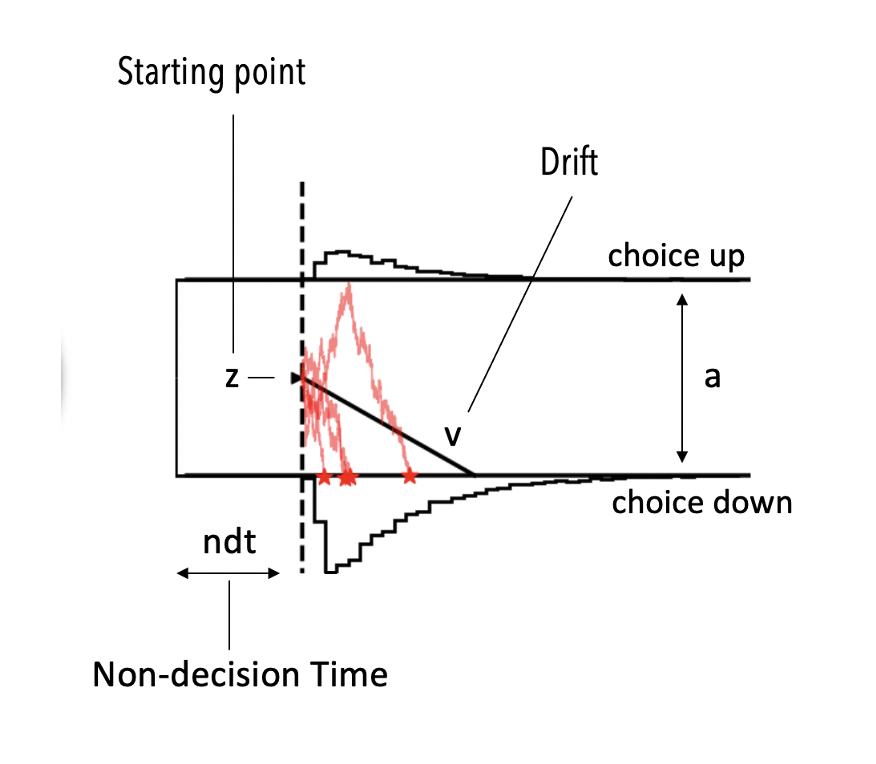
We simulate data with known values first. This makes the later posterior checks concrete: the red reference lines will show the values used to generate the data.
param_dict_init = dict(v=0.5, a=1.5, z=0.5, t=0.5)
v_true, a_true, z_true, t_true = (
    param_dict_init["v"],
    param_dict_init["a"],
    param_dict_init["z"],
    param_dict_init["t"],
)

dataset = hssm.simulate_data(
    model="ddm",
    theta=param_dict_init,
    size=N_SIMPLE_TRIALS,
    random_state=SEEDS["simple"],
)
dataset
| rt | response | |
|---|---|---|
| 0 | 3.145702 | 1.0 |
| 1 | 2.900862 | 1.0 |
| 2 | 1.422539 | 1.0 |
| 3 | 1.330507 | 1.0 |
| 4 | 3.406691 | 1.0 |
| ... | ... | ... |
| 495 | 1.084558 | 1.0 |
| 496 | 1.745612 | 1.0 |
| 497 | 1.136634 | 1.0 |
| 498 | 2.639957 | 1.0 |
| 499 | 2.603419 | 1.0 |
500 rows × 2 columns
Fit the model
To create the simplest HSSM model, provide a pandas.DataFrame with rt and response columns. HSSM supplies the default DDM configuration, including an analytical likelihood and default priors.
What happens in this one line: HSSM checks the data columns, chooses the default DDM parameterization, attaches priors and bounds, and builds the corresponding PyMC model. If you have used HDDM, the workflow will feel familiar. HSSM builds the probabilistic model with PyMC and uses Bambi-style formulas when parameters depend on predictors.
simple_ddm_model = hssm.HSSM(data=dataset, initval_jitter=INITVAL_JITTER)
Model initialized successfully.
simple_ddm_model
Hierarchical Sequential Sampling Model
Model: ddm

Response variable: rt,response
Likelihood: analytical
Observations: 500

Parameters:

v:
    Prior: Normal(mu: 0.0, sigma: 2.0)
    Explicit bounds: (-inf, inf)

a:
    Prior: HalfNormal(sigma: 2.0)
    Explicit bounds: (0.0, inf)

z:
    Prior: Uniform(lower: 0.0, upper: 1.0)
    Explicit bounds: (0.0, 1.0)

t:
    Prior: HalfNormal(sigma: 2.0)
    Explicit bounds: (0.0, inf)


Lapse probability: 0.05
Lapse distribution: Uniform(lower: 0.0, upper: 20.0)
The printed model summary is the first specification check. It shows the observations, free parameters, priors, bounds, and likelihood, so you can confirm that HSSM is estimating the model you intended before spending time sampling.
Inspect the model graph
simple_ddm_model.graph()

The graph uses probabilistic-programming notation:
- white nodes are unknown random variables to estimate;
- the grey node is the observed choice/response-time data;
- rounded rectangles describe dimensions; and
- sharp-cornered rectangles denote deterministic quantities.
For simple models the graph is compact. The goal is not to memorize every node, but to check that the observed data, parameters, and deterministic transformations match your scientific story. The graph becomes especially helpful once regressions and participant-level effects are added.
Sample from the posterior
We now use PyMC's NUTS sampler to draw posterior samples. A posterior sample is a collection of plausible parameter values after combining the prior, the likelihood, and the observed data. The settings below are intentionally small so the tutorial remains runnable; increase chains, draws, and tuning for a real analysis.
infer_data_simple_ddm_model = quiet_call(
    simple_ddm_model.sample,
    sampler="pymc",
    cores=1,
    chains=N_CHAINS,
    draws=N_DRAWS,
    tune=N_TUNE,
    idata_kwargs=dict(log_likelihood=False),
    mp_ctx="spawn",
    progressbar=PYMC_PROGRESS,
    random_seed=SEEDS["simple"],
)
Sampling returns an xarray.DataTree: a labeled container for all the fitted-model results. Next, we will inspect its contents and use ArviZ to assess what the sampler returned.
type(infer_data_simple_ddm_model)
xarray.core.datatree.DataTree
Understand the fitted result
HSSM (via the ArviZ package) stores results in an xarray.DataTree. Each group contains a related part of the Bayesian workflow, such as posterior samples, pointwise log likelihoods, sampler statistics, or observed data.
You do not need to manipulate every group to use HSSM, but recognizing this structure makes it easier to use ArviZ and to add your own analyses. When you see later calls such as az.summary(...), az.plot_trace(...), or az.compare(...), ArviZ is reading these labeled groups.
{
    "groups": tuple(infer_data_simple_ddm_model.children),
    "posterior_sizes": dict(infer_data_simple_ddm_model.posterior.ds.sizes),
}
{'groups': ('posterior', 'sample_stats', 'observed_data'),
 'posterior_sizes': {'chain': 2, 'draw': 500}}
For this model, the most important groups are:
posterior: sampled values for model parameters such asv,a,z, andt;sample_stats: sampler diagnostics such as divergences, tree depth, and acceptance information;observed_data: the choices and response times that were modeled;posterior_predictive: simulated data from the fitted model, added later when we run posterior predictive checks.
This first fit omits log_likelihood to keep the tutorial fast. The three model-comparison fits later enable it because leave-one-out comparison needs trial-level likelihood contributions.
Work with posterior draws
Access groups and variables
tuple(infer_data_simple_ddm_model.posterior.ds.data_vars)
('z', 'a', 't', 'v')
np.round(infer_data_simple_ddm_model.posterior.a.values[0, :5], 3)
array([1.512, 1.481, 1.488, 1.473, 1.524])
To simply access the underlying data as a numpy.ndarray, we can use .values (as e.g. when using pandas.DataFrame objects).
type(infer_data_simple_ddm_model.posterior.a.values)
numpy.ndarray
Combine chains and draws
Many follow-up calculations are easier when the chain and draw dimensions are combined into a single sample dimension. ArviZ's extract helper provides a convenient interface for this common operation. The following cell shows the equivalent lower-level xarray operation.
idata_extracted = az.extract(infer_data_simple_ddm_model)
{
    "variables": tuple(idata_extracted.data_vars),
    "sizes": dict(idata_extracted.sizes),
}
{'variables': ('z', 'a', 't', 'v'), 'sizes': {'sample': 1000}}
dict(infer_data_simple_ddm_model.posterior.ds.stack(sample=("chain", "draw")).sizes)
{'sample': 1000}
ArviZ for diagnostics and visualization

HSSM returns xarray-based inference results that work directly with ArviZ. We will use ArviZ to summarize posterior uncertainty, inspect MCMC traces, check posterior predictions, and compare models. The examples below focus on the few summaries and plots that are most useful when starting out.
Diagnose and interpret the posterior
az.summary(
    infer_data_simple_ddm_model,
    var_names=[var_name.name for var_name in simple_ddm_model.pymc_model.free_RVs],
)
| mean | sd | eti89_lb | eti89_ub | ess_bulk | ess_tail | r_hat | mcse_mean | mcse_sd | |
|---|---|---|---|---|---|---|---|---|---|
| z | 0.516 | 0.019 | 0.49 | 0.55 | 667 | 645 | 1.00 | 0.00074 | 0.00053 |
| a | 1.498 | 0.039 | 1.4 | 1.6 | 576 | 615 | 1.00 | 0.0017 | 0.0012 |
| t | 0.535 | 0.032 | 0.48 | 0.58 | 674 | 586 | 1.00 | 0.0013 | 0.00093 |
| v | 0.493 | 0.045 | 0.42 | 0.57 | 702 | 781 | 1.00 | 0.0017 | 0.0012 |
simple_health = compact_diagnostics(
    infer_data_simple_ddm_model,
    var_names=["v", "a", "z", "t"],
)
if FULL_RUN:
    assert simple_health["divergence_rate"] <= 0.005, (
        "core DDM divergence rate exceeds 0.5%"
    )
    assert simple_health["max_rhat"] <= 1.01, (
        f"core DDM max R-hat is {simple_health['max_rhat']:.4f}"
    )
    assert simple_health["min_bulk_or_tail_ess"] >= 200, (
        "core DDM minimum bulk/tail ESS is below 200"
    )
simple_health
{'scope': 'full diagnostic validation',
 'divergences': 0,
 'divergence_rate': 0.0,
 'max_rhat': 1.0042907918737856,
 'min_bulk_or_tail_ess': 576.3121233231101}
The summary reports posterior location and uncertainty for each parameter, plus diagnostics. The mean and sd columns describe the center and spread of the posterior draws. The highest-density interval (hdi_3% to hdi_97% by default) gives a compact uncertainty interval. Start diagnostics with r_hat: values near 1 indicate that independent chains explored the same distribution. As a practical rule, investigate values above 1.01 and inspect trace plots before interpreting parameter estimates.
Trace and distribution plots
_pc = az.plot_trace_dist(infer_data_simple_ddm_model)
add_trace_reference_lines(_pc, param_dict_init)

HSSM also stores the latest result on .traces. Both access patterns are equivalent; this reactive notebook keeps using the explicitly returned result so every diagnostic has a visible dependency on sampling.
The distribution panel summarizes posterior uncertainty for each parameter. The MCMC trace panel shows each chain across draws; stable, overlapping chains suggest the sampler is repeatedly visiting the same high-probability region rather than getting stuck in different places. The red reference lines mark the known values used to simulate the data.
Forest plots
_ = az.plot_forest(infer_data_simple_ddm_model)

A forest plot turns posterior uncertainty into intervals, which is useful when many parameters or chains are shown at once. By default, chains are shown separately. Combining chains can make a large forest plot easier to scan once you have already checked trace diagnostics.
_ = az.plot_forest(infer_data_simple_ddm_model, combined=True)

Marginal posterior plots
A marginal posterior plot ignores sampling order and focuses on the distribution of one parameter at a time. Because this is simulated data, we can compare the posterior with the known generating values. The standalone marginal plot below uses vertical reference lines; the paired trace/distribution plots use vertical lines on distributions and horizontal lines on traces.
_pc = az.plot_dist(infer_data_simple_ddm_model, kind="hist")
_ = az.add_lines(
    _pc,
    values=param_dict_init,
    orientation="vertical",
    visuals={"ref_line": dict(color="red", linestyle="--")},
)

Posterior pair plots
Pair plots reveal relationships between posterior parameters. Strong trade-offs can signal weak identification: when one parameter increases, another may compensate while producing similar predicted behavior. This is common in cognitive models, where several parameters can affect the same response-time or choice pattern.
_ = az.plot_pair(infer_data_simple_ddm_model, marginal_kind="kde")

ArviZ provides many additional diagnostics and plotting tools. The current user guide is the best next reference when you need a specific plot or diagnostic.
Compute quantities from posterior draws
# Calculate the correlation matrix
posterior_correlation_matrix = np.corrcoef(
    np.stack(
        [idata_extracted[var_].values for var_ in idata_extracted.data_vars.variables]
    )
)
num_vars = posterior_correlation_matrix.shape[0]
fig, ax = plt.subplots(1, 1)
cax = ax.imshow(posterior_correlation_matrix, cmap="coolwarm", vmin=-1, vmax=1)
fig.colorbar(cax, ax=ax)
ax.set_title("Posterior Correlation Matrix")
ax.set_xticks(range(posterior_correlation_matrix.shape[0]))
# Make heatmap
ax.set_xticklabels([var_ for var_ in idata_extracted.data_vars.variables])
ax.set_yticks(range(posterior_correlation_matrix.shape[0]))
ax.set_yticklabels([var_ for var_ in idata_extracted.data_vars.variables])
for _i in range(num_vars):
    for j in range(num_vars):
        # Add ticks
        ax.text(
            j,
            _i,
            f"{posterior_correlation_matrix[_i, j]:.2f}",
            ha="center",
            va="center",
            color="black",
        )
# Annotate heatmap
plt.show()

Check posterior predictions
Good MCMC diagnostics show that the sampler explored the stated model reliably; they do not show that the model captures the data. Posterior predictive checks compare data simulated from the fitted model with the observations and are an essential step before substantive interpretation. In workflow terms, this is where we ask: if the fitted model were true, would it generate choices and response times that look like the data we actually observed?
ppc_idata = quiet_call(
    simple_ddm_model.sample_posterior_predictive,
    dt=infer_data_simple_ddm_model,
    draws=N_PPC_DRAWS,
    inplace=False,
)
Warning: Numba will use object mode to run ddm_RV_rv{"(),(),(),(),()->(2)"}'s perform method. Set `pytensor.config.compiler_verbose = True` to see more details.
_ppc_axes = simple_ddm_model.plot_predictive(dt=ppc_idata)
_ppc_figure = _ppc_axes.figure
plt.close(_ppc_figure)
_ppc_figure

The posterior predictive call returns a result with a posterior_predictive group, and plot_predictive() visualizes those simulated datasets against the observations. If predictions reproduce the main features of the observed response-time and choice distributions, the model is a useful approximation for those features. Systematic mismatches suggest revisiting the likelihood, parameterization, covariates, or model family.
HSSM does not currently expose a random-seed argument for posterior predictive sampling. All data simulation and MCMC fits on this page are seeded; the exact predictive draws may vary while the same model check is performed.
2. Choose a model and likelihood
simple_ddm_model.loglik_kind
'analytical'
The DDM above used HSSM’s analytical likelihood. Other sequential-sampling models may instead use an approx_differentiable likelihood, such as a likelihood approximation network (LAN), or a user-supplied blackbox likelihood. The model interface stays similar; HSSM chooses compatible computational machinery behind the scenes.
An angle model with collapsing boundaries
The angle model extends the DDM with theta, which controls the rate at which decision boundaries collapse over time.
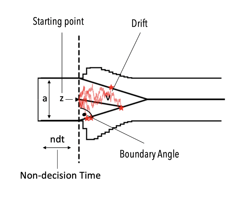
Collapsing boundaries are useful when urgency or time pressure may change a participant’s decision criterion. HSSM makes inference for these models practical through packaged approx_differentiable likelihoods.
# Simulate angle data
v_angle_true = 0.5
a_angle_true = 1.5
z_angle_true = 0.5
t_angle_true = 0.2
theta_angle_true = 0.2

param_dict_angle = dict(v=0.5, a=1.5, z=0.5, t=0.2, theta=0.2)

dataset_angle = hssm.simulate_data(
    model="angle",
    theta=param_dict_angle,
    size=N_ANGLE_TRIALS,
    random_state=SEEDS["angle"],
)
We pass a single additional argument to our HSSM class and set model='angle'.
model_angle = hssm.HSSM(
    data=dataset_angle, model="angle", initval_jitter=INITVAL_JITTER
)

model_angle
Warning: You are sending unauthenticated requests to the HF Hub. Please set a HF_TOKEN to enable higher rate limits and faster downloads.
Model initialized successfully.
Hierarchical Sequential Sampling Model
Model: angle

Response variable: rt,response
Likelihood: approx_differentiable
Observations: 1000

Parameters:

v:
    Prior: Uniform(lower: -3.0, upper: 3.0)
    Explicit bounds: (-3.0, 3.0)

a:
    Prior: Uniform(lower: 0.3, upper: 3.0)
    Explicit bounds: (0.3, 3.0)

z:
    Prior: Uniform(lower: 0.1, upper: 0.9)
    Explicit bounds: (0.1, 0.9)

t:
    Prior: Uniform(lower: 0.001, upper: 2.0)
    Explicit bounds: (0.001, 2.0)

theta:
    Prior: Uniform(lower: -0.1, upper: 1.3)
    Explicit bounds: (-0.1, 1.3)


Lapse probability: 0.05
Lapse distribution: Uniform(lower: 0.0, upper: 20.0)
The graph now includes the additional theta parameter. This is a quick way to confirm that the model specification matches the scientific question.
model_angle.graph()

Let's check the type of likelihood that is used under the hood ...
model_angle.loglik_kind
'approx_differentiable'
This model uses an approx_differentiable likelihood. In the packaged model collection, that typically means a LAN is used internally to approximate the likelihood.
jax.config.update("jax_enable_x64", False)
infer_data_angle = quiet_call(
    model_angle.sample,
    sampler="numpyro",
    chains=N_CHAINS,
    cores=1,
    draws=N_DRAWS,
    tune=N_TUNE,
    idata_kwargs=dict(log_likelihood=False),  # no need to return likelihoods here
    # mp_ctx="spawn",
    progressbar=EXTERNAL_PROGRESS,
    random_seed=SEEDS["angle"],
)
Warning: `init='adapt_diag'` is ignored by `nuts_sampler='numpyro'`; the external sampler uses its own initialization.
Warning: There are not enough devices to run parallel chains: expected 2 but got 1. Chains will be drawn sequentially. If you are running MCMC in CPU, consider using `numpyro.set_host_device_count(2)` at the beginning of your program. You can double-check how many devices are available in your system using `jax.local_device_count()`.
Warning: Explicitly requested dtype float64 requested in astype is not available, and will be truncated to dtype float32. To enable more dtypes, set the jax_enable_x64 configuration option or the JAX_ENABLE_X64 shell environment variable. See https://github.com/jax-ml/jax#current-gotchas for more.
_pc = az.plot_trace_dist(infer_data_angle)
add_trace_reference_lines(_pc, param_dict_angle)

3. Customize priors and model structure
Priors express plausible parameter ranges before observing the data. HSSM supports defaults that respect model bounds, fixed values for parameters you do not want to estimate, and explicit PyMC distributions when you need stronger domain knowledge.
Fix parameters when the design justifies it
Sometimes a parameter is fixed by design or is outside the present research question. Here we estimate only the drift rate v while holding the other DDM parameters fixed.
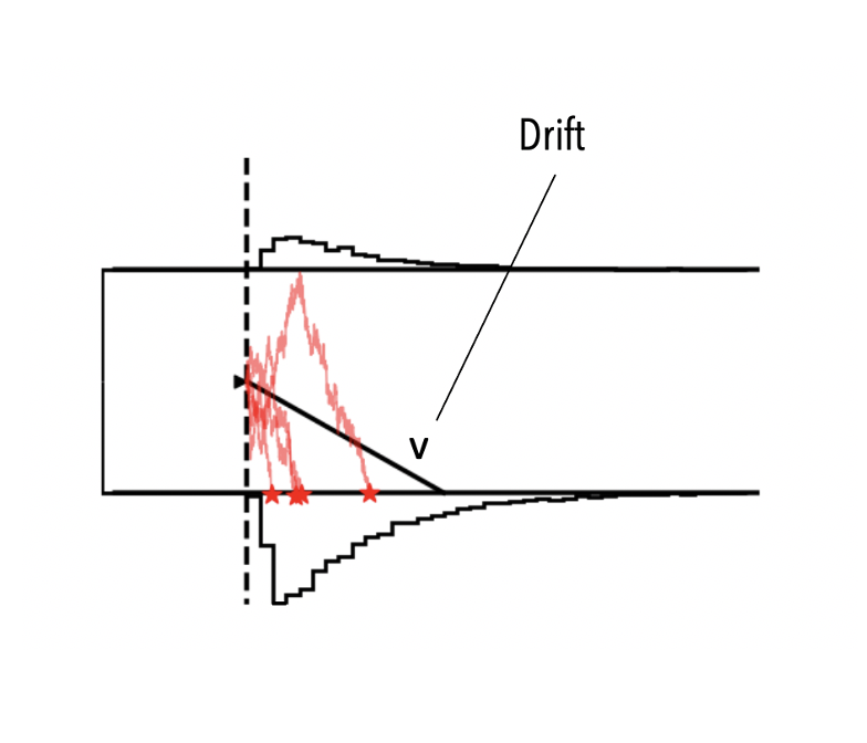
Fixing parameters reduces model flexibility, so it should be justified by theory, design, or a deliberate comparison.
param_dict_init
{'v': 0.5, 'a': 1.5, 'z': 0.5, 't': 0.5}
ddm_model_only_v = hssm.HSSM(
    data=dataset,
    model="ddm",
    a=param_dict_init["a"],
    t=param_dict_init["t"],
    z=param_dict_init["z"],
    initval_jitter=INITVAL_JITTER,
)
Model initialized successfully.
Since we fix all but one parameter, we estimate only one parameter. This is a useful pattern when a parameter is known from design, when a previous analysis justifies a fixed value, or when you want to isolate one cognitive process. The model graph should reflect this choice: we expect only one free random variable, v.
ddm_model_only_v.graph()

infer_data_only_v = quiet_call(
    ddm_model_only_v.sample,
    sampler="pymc",
    chains=N_CHAINS,
    cores=1,
    draws=N_PRIMARY_REG_DRAWS,
    tune=N_PRIMARY_REG_TUNE,
    idata_kwargs=dict(log_likelihood=False),  # no need to return likelihoods here
    mp_ctx="spawn",
    progressbar=PYMC_PROGRESS,
    random_seed=SEEDS["only_v"],
)
_pc = az.plot_trace_dist(infer_data_only_v)
add_trace_reference_lines(_pc, {"v": param_dict_init["v"]})

A rank plot complements a trace plot by checking whether chains are sampling from the same distribution. Roughly uniform ranks across chains are consistent with good mixing; visible chain-specific patterns call for further diagnosis.
if FULL_RUN:
    _ = az.plot_rank(infer_data_only_v)
else:
    print("Rank diagnostics require the two-chain full run.")

Specify informative priors
model_normal = hssm.HSSM(
    data=dataset,
    include=[
        {
            "name": "v",
            "prior": {"name": "Normal", "mu": 0, "sigma": 0.01},
        }
    ],
    initval_jitter=INITVAL_JITTER,
)
Model initialized successfully.
model_normal
Hierarchical Sequential Sampling Model
Model: ddm

Response variable: rt,response
Likelihood: analytical
Observations: 500

Parameters:

v:
    Prior: Normal(mu: 0.0, sigma: 0.01)
    Explicit bounds: (-inf, inf)

a:
    Prior: HalfNormal(sigma: 2.0)
    Explicit bounds: (0.0, inf)

z:
    Prior: Uniform(lower: 0.0, upper: 1.0)
    Explicit bounds: (0.0, 1.0)

t:
    Prior: HalfNormal(sigma: 2.0)
    Explicit bounds: (0.0, inf)


Lapse probability: 0.05
Lapse distribution: Uniform(lower: 0.0, upper: 20.0)
infer_data_normal = quiet_call(
    model_normal.sample,
    sampler="pymc",
    chains=N_CHAINS,
    cores=1,
    draws=N_DRAWS,
    tune=N_TUNE,
    idata_kwargs=dict(log_likelihood=False),  # no need to return likelihoods here
    mp_ctx="spawn",
    progressbar=PYMC_PROGRESS,
    random_seed=SEEDS["bad_prior"],
)
_pc = az.plot_trace_dist(infer_data_normal)
add_trace_reference_lines(_pc, param_dict_init)

narrow_prior_health = compact_diagnostics(
    infer_data_normal,
    var_names=["v", "a", "z", "t"],
)
narrow_prior_health
{'scope': 'full diagnostic validation',
 'divergences': 0,
 'divergence_rate': 0.0,
 'max_rhat': 1.0035265663892592,
 'min_bulk_or_tail_ess': 458.21280608936786}
The data were generated with v=0.5, a=1.5, z=0.5, and t=0.5. Compare the trace and compact diagnostic snapshot with the baseline fit. If the narrow prior pulls v toward zero, other parameters may compensate; any divergences or weak diagnostics are reasons not to interpret this intentionally restrictive fit. This example is reported, not gated, because it is designed to illustrate a problematic prior.
Regressions on cognitive parameters

HSSM can link individual SSM parameters to trial-level covariates with Bambi-style formulas. This lets you ask questions such as whether a neural signal, condition, or behavioral measure predicts drift rate, boundary separation, or bias.
One parameter as a regression target
Simulating Data
We simulate data in which drift rate varies with two trial-level covariates. The known coefficients give us a clear recovery target.
# Set up trial by trial parameters
_rng = np.random.default_rng(SEEDS["reg"])
v_intercept = 0.3
x = _rng.uniform(-1, 1, size=N_REG_TRIALS)
v_x = 0.8
y = _rng.uniform(-1, 1, size=N_REG_TRIALS)
v_y = 0.3
_v_reg_v = v_intercept + v_x * x + v_y * y
_a_reg_v = 1.5
# rest
_z_reg_v = 0.5
_t_reg_v = 0.1
param_dict_reg_v = dict(
    a=1.5,
    z=0.5,
    t=0.1,
    v=_v_reg_v,
    v_x=v_x,
    v_y=v_y,
    v_Intercept=v_intercept,
    theta=0.0,
)
dataset_reg_v = hssm.simulate_data(
    model="ddm",
    theta=param_dict_reg_v,
    size=1,
    random_state=SEEDS["reg"],
)
dataset_reg_v["x"] = x
# base dataset
# Adding covariates into the datsaframe
dataset_reg_v["y"] = y
Define the regression
The include argument contains one specification per parameter with a regression. Each specification names the parameter, supplies a formula and link, and can define priors for regression coefficients.
Formula syntax follows Bambi and familiar R-style mixed-model notation. HSSM uses Bambi to translate these formulas into a PyMC model. Conceptually, this means the SSM parameter is no longer a single value; it can vary systematically with trial-level or participant-level predictors.
model_reg_v_simple = hssm.HSSM(
    data=dataset_reg_v,
    include=[{"name": "v", "formula": "v ~ 1 + x + y"}],
    initval_jitter=INITVAL_JITTER,
)
Model initialized successfully.
Param class
As illustrated below, there is an alternative way of specifying the parameter specific data via the Param class.
model_reg_v_simple_new = hssm.HSSM(
    data=dataset_reg_v,
    include=[hssm.Param(name="v", formula="v ~ 1 + x + y")],
    initval_jitter=INITVAL_JITTER,
)
Model initialized successfully.
{
    "dict_specification_free_RVs": tuple(
        rv.name for rv in model_reg_v_simple.pymc_model.free_RVs
    ),
    "Param_specification_free_RVs": tuple(
        rv.name for rv in model_reg_v_simple_new.pymc_model.free_RVs
    ),
}
{'dict_specification_free_RVs': ('z', 'a', 't', 'v_Intercept', 'v_x', 'v_y'),
 'Param_specification_free_RVs': ('z', 'a', 't', 'v_Intercept', 'v_x', 'v_y')}
model_reg_v_simple.graph()

Customize parameter-specific priors
The default regression specification is often a good starting point. When prior knowledge is available, specify coefficient-level priors explicitly and then verify the resulting model summary before sampling.
model_reg_v = hssm.HSSM(
    data=dataset_reg_v,
    include=[
        {
            "name": "v",
            "prior": {
                "Intercept": {"name": "Uniform", "lower": -3.0, "upper": 3.0},
                "x": {"name": "Uniform", "lower": -1.0, "upper": 1.0},
                "y": {"name": "Uniform", "lower": -1.0, "upper": 1.0},
            },
            "formula": "v ~ 1 + x + y",
            "link": "identity",
        }
    ],
    initval_jitter=INITVAL_JITTER,
)
Model initialized successfully.
model_reg_v
Hierarchical Sequential Sampling Model
Model: ddm

Response variable: rt,response
Likelihood: analytical
Observations: 1000

Parameters:

v:
    Formula: v ~ 1 + x + y
    Priors:
        v_Intercept ~ Uniform(lower: -3.0, upper: 3.0)
        v_x ~ Uniform(lower: -1.0, upper: 1.0)
        v_y ~ Uniform(lower: -1.0, upper: 1.0)
    Link: identity
    Explicit bounds: (-inf, inf)

a:
    Prior: HalfNormal(sigma: 2.0)
    Explicit bounds: (0.0, inf)

z:
    Prior: Uniform(lower: 0.0, upper: 1.0)
    Explicit bounds: (0.0, 1.0)

t:
    Prior: HalfNormal(sigma: 2.0)
    Explicit bounds: (0.0, inf)


Lapse probability: 0.05
Lapse distribution: Uniform(lower: 0.0, upper: 20.0)
The model summary now shows v as a regression with an intercept and covariate coefficients. This is the same specification-check step as before, but now the summary should also confirm that the intended predictors entered the model.
infer_data_reg_v = quiet_call(
    model_reg_v.sample,
    sampler="pymc",
    chains=N_CHAINS,
    cores=1,
    draws=N_PRIMARY_REG_DRAWS,
    tune=N_PRIMARY_REG_TUNE,
    idata_kwargs={"log_likelihood": False},
    mp_ctx="spawn",
    progressbar=PYMC_PROGRESS,
    random_seed=SEEDS["reg"],
)
az.summary(infer_data_reg_v, var_names=["~a", "~z", "~t"])
| mean | sd | eti89_lb | eti89_ub | ess_bulk | ess_tail | r_hat | mcse_mean | mcse_sd | |
|---|---|---|---|---|---|---|---|---|---|
| v_x | 0.857 | 0.049 | 0.78 | 0.94 | 1115 | 755 | 1.00 | 0.0015 | 0.001 |
| v_y | 0.371 | 0.046 | 0.3 | 0.44 | 1613 | 1028 | 1.00 | 0.0011 | 0.00082 |
| v_Intercept | 0.325 | 0.032 | 0.27 | 0.38 | 1048 | 959 | 1.00 | 0.001 | 0.00068 |
_pc = az.plot_trace_dist(
    infer_data_reg_v,
    var_names=["v_Intercept", "v_x", "v_y", "a", "z", "t"],
)
add_trace_reference_lines(_pc, param_dict_reg_v)

regression_health = compact_diagnostics(
    infer_data_reg_v,
    var_names=["v_Intercept", "v_x", "v_y", "a", "z", "t"],
)
recovery_report = {}
raw_hdis = {}
probabilities_positive = {}
for _name in ("v_Intercept", "v_x", "v_y"):
    _draws = az.extract(infer_data_reg_v, var_names=[_name]).values
    _hdi = az.hdi(_draws, prob=0.94)
    raw_hdis[_name] = _hdi
    probabilities_positive[_name] = float((_draws > 0).mean())
    recovery_report[_name] = {
        "known_value": param_dict_reg_v[_name],
        "posterior_mean": round(float(_draws.mean()), 3),
        "94%_HDI": tuple(round(float(value), 3) for value in _hdi),
        "P(>0)": round(probabilities_positive[_name], 3),
    }
if FULL_RUN:
    assert regression_health["divergence_rate"] <= 0.005, (
        "primary regression divergence rate exceeds 0.5%"
    )
    assert regression_health["max_rhat"] <= 1.01, (
        f"primary regression max R-hat is {regression_health['max_rhat']:.4f}"
    )
    assert regression_health["min_bulk_or_tail_ess"] >= 200, (
        "primary regression minimum bulk/tail ESS is below 200"
    )
    _v_x_hdi = raw_hdis["v_x"]
    assert _v_x_hdi[0] <= param_dict_reg_v["v_x"] <= _v_x_hdi[1], (
        "primary regression HDI misses the known focal v_x effect"
    )
    assert probabilities_positive["v_x"] >= 0.95, (
        "primary regression does not clearly support a positive v_x effect"
    )
{"diagnostics": regression_health, "coefficient_recovery": recovery_report}
{'diagnostics': {'scope': 'full diagnostic validation',
  'divergences': 0,
  'divergence_rate': 0.0,
  'max_rhat': 1.0044706337239624,
  'min_bulk_or_tail_ess': 755.3872223026837},
 'coefficient_recovery': {'v_Intercept': {'known_value': 0.3,
   'posterior_mean': 0.325,
   '94%_HDI': (0.264, 0.384),
   'P(>0)': 1.0},
  'v_x': {'known_value': 0.8,
   'posterior_mean': 0.857,
   '94%_HDI': (0.77, 0.958),
   'P(>0)': 1.0},
  'v_y': {'known_value': 0.3,
   'posterior_mean': 0.371,
   '94%_HDI': (0.283, 0.452),
   'P(>0)': 1.0}}}
The full publication run requires acceptable diagnostics and checks that the 94% interval for the focal v_x coefficient contains its known value (0.8) with high posterior probability above zero. The intercept and v_y estimates are reported without simultaneous-coverage assertions; inspect their uncertainty rather than treating every finite simulation as exact recovery.
Regression with an angle model
model_reg_v_angle = hssm.HSSM(
    data=dataset_reg_v,
    model="angle",
    include=[
        {
            "name": "v",
            "prior": {
                "Intercept": {
                    "name": "Uniform",
                    "lower": -3.0,
                    "upper": 3.0,
                },
                "x": {
                    "name": "Uniform",
                    "lower": -1.0,
                    "upper": 1.0,
                },
                "y": {"name": "Uniform", "lower": -1.0, "upper": 1.0},
            },
            "formula": "v ~ 1 + x + y",
            "link": "identity",
        }
    ],
    initval_jitter=INITVAL_JITTER,
)
Model initialized successfully.
model_reg_v_angle.graph()

trace_reg_v_angle = quiet_call(
    model_reg_v_angle.sample,
    sampler="pymc",
    chains=N_CHAINS,
    cores=1,
    draws=N_DRAWS,
    tune=N_TUNE,
    idata_kwargs={"log_likelihood": False},
    mp_ctx="spawn",
    progressbar=PYMC_PROGRESS,
    random_seed=SEEDS["reg_angle"],
)
Warning: Numba will use object mode to run LANLogpOp's perform method. Set `pytensor.config.compiler_verbose = True` to see more details.
Warning: Numba will use object mode to run LANLogpVJPOp's perform method. Set `pytensor.config.compiler_verbose = True` to see more details.
_pc = az.plot_trace_dist(
    trace_reg_v_angle,
    var_names=["v_Intercept", "v_x", "v_y", "a", "z", "t", "theta"],
)
add_trace_reference_lines(_pc, param_dict_reg_v)

Inspect the posterior interval for theta: data generated by a standard DDM support the expected story only when that interval is compatible with zero and the sampler diagnostics are acceptable. Interpret the remaining parameters with the same conditional workflow.
Regress multiple parameters
We now fit regressions for both v and a. Only v truly varies with the simulated covariates, so the a coefficients should be centered near zero.
# Instantiate our hssm model
from copy import deepcopy

param_dict_reg_v_a = deepcopy(param_dict_reg_v)
param_dict_reg_v_a["a_Intercept"] = param_dict_reg_v_a["a"]
param_dict_reg_v_a["a_x"] = 0
param_dict_reg_v_a["a_y"] = 0

hssm_reg_v_a_angle = hssm.HSSM(
    data=dataset_reg_v,
    model="angle",
    include=[
        {
            "name": "v",
            "prior": {
                "Intercept": {"name": "Uniform", "lower": -3.0, "upper": 3.0},
                "x": {"name": "Uniform", "lower": -1.0, "upper": 1.0},
                "y": {"name": "Uniform", "lower": -1.0, "upper": 1.0},
            },
            "formula": "v ~ 1 + x + y",
        },
        {
            "name": "a",
            "prior": {
                "Intercept": {"name": "Uniform", "lower": 0.5, "upper": 3.0},
                "x": {"name": "Uniform", "lower": -1.0, "upper": 1.0},
                "y": {"name": "Uniform", "lower": -1.0, "upper": 1.0},
            },
            "formula": "a ~ 1 + x + y",
        },
    ],
    initval_jitter=INITVAL_JITTER,
)
Model initialized successfully.
hssm_reg_v_a_angle
Hierarchical Sequential Sampling Model
Model: angle

Response variable: rt,response
Likelihood: approx_differentiable
Observations: 1000

Parameters:

v:
    Formula: v ~ 1 + x + y
    Priors:
        v_Intercept ~ Uniform(lower: -3.0, upper: 3.0)
        v_x ~ Uniform(lower: -1.0, upper: 1.0)
        v_y ~ Uniform(lower: -1.0, upper: 1.0)
    Link: identity
    Explicit bounds: (-3.0, 3.0)

a:
    Formula: a ~ 1 + x + y
    Priors:
        a_Intercept ~ Uniform(lower: 0.5, upper: 3.0)
        a_x ~ Uniform(lower: -1.0, upper: 1.0)
        a_y ~ Uniform(lower: -1.0, upper: 1.0)
    Link: identity
    Explicit bounds: (0.3, 3.0)

z:
    Prior: Uniform(lower: 0.1, upper: 0.9)
    Explicit bounds: (0.1, 0.9)

t:
    Prior: Uniform(lower: 0.001, upper: 2.0)
    Explicit bounds: (0.001, 2.0)

theta:
    Prior: Uniform(lower: -0.1, upper: 1.3)
    Explicit bounds: (-0.1, 1.3)


Lapse probability: 0.05
Lapse distribution: Uniform(lower: 0.0, upper: 20.0)
hssm_reg_v_a_angle.graph()

infer_data_reg_v_a = quiet_call(
    hssm_reg_v_a_angle.sample,
    sampler="pymc",
    chains=N_CHAINS,
    cores=1,
    draws=N_DRAWS,
    tune=N_TUNE,
    idata_kwargs={"log_likelihood": False},
    mp_ctx="spawn",
    progressbar=PYMC_PROGRESS,
    random_seed=SEEDS["reg_multi"],
)
Warning: Numba will use object mode to run LANLogpOp's perform method. Set `pytensor.config.compiler_verbose = True` to see more details.
Warning: Numba will use object mode to run LANLogpVJPOp's perform method. Set `pytensor.config.compiler_verbose = True` to see more details.
az.summary(
    infer_data_reg_v_a,
    var_names=[
        "v_Intercept",
        "v_x",
        "v_y",
        "a_Intercept",
        "a_x",
        "a_y",
        "z",
        "t",
        "theta",
    ],
)
| mean | sd | eti89_lb | eti89_ub | ess_bulk | ess_tail | r_hat | mcse_mean | mcse_sd | |
|---|---|---|---|---|---|---|---|---|---|
| v_Intercept | 0.317 | 0.034 | 0.26 | 0.37 | 850 | 870 | 1.00 | 0.0012 | 0.00074 |
| v_x | 0.857 | 0.052 | 0.78 | 0.94 | 919 | 536 | 1.00 | 0.0017 | 0.001 |
| v_y | 0.364 | 0.047 | 0.29 | 0.44 | 1197 | 762 | 1.00 | 0.0014 | 0.00097 |
| a_Intercept | 1.438 | 0.044 | 1.4 | 1.5 | 519 | 516 | 1.00 | 0.0019 | 0.0013 |
| a_x | 0.016 | 0.037 | -0.041 | 0.076 | 1052 | 781 | 1.00 | 0.0011 | 0.00086 |
| a_y | -0.022 | 0.036 | -0.082 | 0.034 | 1112 | 742 | 1.00 | 0.0011 | 0.00079 |
| z | 0.5055 | 0.0121 | 0.49 | 0.52 | 769 | 774 | 1.00 | 0.00044 | 0.0003 |
| t | 0.129 | 0.022 | 0.093 | 0.16 | 534 | 453 | 1.00 | 0.00097 | 0.0007 |
| theta | 0.022 | 0.02 | -0.011 | 0.056 | 568 | 616 | 1.00 | 0.00086 | 0.00059 |
_pc = az.plot_trace_dist(
    infer_data_reg_v_a,
    var_names=[
        "v_Intercept",
        "v_x",
        "v_y",
        "a_Intercept",
        "a_x",
        "a_y",
        "z",
        "t",
        "theta",
    ],
)
add_trace_reference_lines(_pc, param_dict_reg_v_a)

Use the numeric summary to assess recovery: the v rows should be compared with their known coefficients, while the a_x and a_y intervals should be checked for compatibility with zero because the data-generating process did not vary a with these covariates. Treat either pattern as evidence from this finite run, not a guaranteed outcome.
Categorical covariates
_rng = np.random.default_rng(SEEDS["categorical"])
x_1 = _rng.choice(4, size=N_REG_TRIALS).astype(int)
x_offset = np.array([0, 1, -0.5, 0.75])
y_1 = _rng.uniform(-1, 1, size=N_REG_TRIALS)
v_y_1 = 0.3
_v_reg_v = 0 + v_y_1 * y_1 + x_offset[x_1]
_a_reg_v = 1.5
_z_reg_v = 0.5
_t_reg_v = 0.1
dataset_reg_v_cat = hssm.simulate_data(
    model="ddm",
    theta=dict(v=_v_reg_v, a=_a_reg_v, z=_z_reg_v, t=_t_reg_v),
    size=1,
    random_state=SEEDS["categorical"],
)
dataset_reg_v_cat["x"] = x_1
dataset_reg_v_cat["y"] = y_1
model_reg_v_cat = hssm.HSSM(
    data=dataset_reg_v_cat,
    model="angle",
    include=[
        {
            "name": "v",
            "formula": "v ~ 0 + C(x) + y",
            "link": "identity",
        }
    ],
    initval_jitter=INITVAL_JITTER,
)
Model initialized successfully.
model_reg_v_cat.graph()

infer_data_reg_v_cat = quiet_call(
    model_reg_v_cat.sample,
    sampler="pymc",
    chains=N_CHAINS,
    cores=1,
    draws=N_DRAWS,
    tune=N_TUNE,
    idata_kwargs={"log_likelihood": False},
    mp_ctx="spawn",
    progressbar=PYMC_PROGRESS,
    random_seed=SEEDS["categorical"],
)
Warning: Numba will use object mode to run LANLogpOp's perform method. Set `pytensor.config.compiler_verbose = True` to see more details.
Warning: Numba will use object mode to run LANLogpVJPOp's perform method. Set `pytensor.config.compiler_verbose = True` to see more details.
_ = az.plot_forest(infer_data_reg_v_cat)

Hierarchical participant effects
Next we simulate data from 15 participants, each with 200 trials. A hierarchy lets participant-level estimates share information through a group distribution while preserving individual differences.
Simulate Data
_rng = np.random.default_rng(SEEDS["hier"])
n_participants = N_HIER_PARTICIPANTS
n_trials = N_HIER_TRIALS
sd_v = 0.5
mean_v = 0.5
data_list = []
for _i in range(n_participants):
    v_intercept_hier = _rng.normal(mean_v, sd_v, size=1)
    x_2 = _rng.uniform(-1, 1, size=n_trials)
    v_x_hier = 0.8
    y_2 = _rng.uniform(-1, 1, size=n_trials)
    v_y_hier = 0.3
    v_hier = v_intercept_hier + v_x_hier * x_2 + v_y_hier * y_2
    a_hier = 1.5
    t_hier = 0.5
    z_hier = 0.5
    data_tmp = hssm.simulate_data(
        model="ddm",
        theta=dict(v=v_hier, a=a_hier, z=z_hier, t=t_hier),
        size=1,
        random_state=SEEDS["hier"] + _i,
    )
    data_tmp["participant_id"] = _i
    data_tmp["x"] = x_2
    data_tmp["y"] = y_2
    data_list.append(data_tmp)
dataset_reg_v_hier = pd.concat(data_list)
dataset_reg_v_hier
| rt | response | participant_id | x | y | |
|---|---|---|---|---|---|
| 0 | 1.804934 | -1.0 | 0 | -0.785018 | 0.792162 |
| 1 | 3.947494 | 1.0 | 0 | 0.295662 | -0.817377 |
| 2 | 1.259359 | 1.0 | 0 | 0.921396 | 0.082609 |
| 3 | 1.769029 | 1.0 | 0 | 0.540598 | 0.916793 |
| 4 | 3.031497 | 1.0 | 0 | 0.816505 | -0.200228 |
| ... | ... | ... | ... | ... | ... |
| 195 | 1.701335 | 1.0 | 14 | 0.269187 | 0.508749 |
| 196 | 4.755053 | 1.0 | 14 | 0.573819 | 0.963991 |
| 197 | 1.670578 | 1.0 | 14 | 0.427159 | -0.728222 |
| 198 | 0.943260 | -1.0 | 14 | -0.029444 | 0.833860 |
| 199 | 1.775628 | 1.0 | 14 | 0.506406 | 0.901653 |
3000 rows × 5 columns
We use v ~ 1 + (1|participant_id) + x + y. The random-intercept term (1|participant_id) gives each participant an offset around the group intercept; the remaining coefficients are shared across participants. The hierarchy lets participants borrow strength from the group while still allowing individual differences.
Basic Hierarchical Model
Note the noncentered=True argument below: it selects the non-centered parameterization for the group-specific terms. The default is the right choice here — when and why to flip it (globally, or per parameter) is covered in Centered vs. non-centered parameterizations and Per-parameter parameterization.
model_reg_v_angle_hier = hssm.HSSM(
    data=dataset_reg_v_hier,
    model="angle",
    noncentered=True,
    initval_jitter=INITVAL_JITTER,
    include=[
        {
            "name": "v",
            "prior": {
                "Intercept": {
                    "name": "Normal",
                    "mu": 0.0,
                    "sigma": 0.5,
                },
                "x": {"name": "Normal", "mu": 0.0, "sigma": 0.5},
                "y": {"name": "Normal", "mu": 0.0, "sigma": 0.5},
            },
            "formula": "v ~ 1 + (1|participant_id) + x + y",
            "link": "identity",
        }
    ],
)
Model initialized successfully.
model_reg_v_angle_hier.graph()

jax.config.update("jax_enable_x64", False)
infer_data_reg_v_angle_hier = quiet_call(
    model_reg_v_angle_hier.sample,
    sampler="pymc",
    chains=N_CHAINS,
    cores=1,
    draws=N_DRAWS,
    tune=N_TUNE,
    idata_kwargs={"log_likelihood": False},
    mp_ctx="spawn",
    progressbar=PYMC_PROGRESS,
    random_seed=SEEDS["hier"],
)
Warning: Numba will use object mode to run LANLogpOp's perform method. Set `pytensor.config.compiler_verbose = True` to see more details.
Warning: Numba will use object mode to run LANLogpVJPOp's perform method. Set `pytensor.config.compiler_verbose = True` to see more details.
Inspect the posterior to distinguish group-level effects from participant-level variation and to confirm that the chains mix well. In hierarchical models, it is especially useful to separate population-level parameters from participant-specific offsets before interpreting the substantive effects.
_ = az.plot_forest(infer_data_reg_v_angle_hier, combined=False)

4. Validate and compare models
Model comparison asks how well competing models predict the same data while accounting for fit and complexity. It comes after diagnostics and posterior predictive checks because a model with poor sampling behavior or obvious predictive failures is not a strong scientific candidate, even if a comparison table looks favorable. Here the data are generated with a=1.5, and we compare three DDMs that fix a too low (1.3), correctly (1.5), or too high (1.7).
We use ArviZ's compare() function with expected log predictive density from leave-one-out cross-validation (elpd_loo). Higher expected predictive accuracy is better, but close differences should be interpreted as uncertainty rather than a hard ranking.
Data Simulation
# Parameters
param_dict_mod_comp = dict(v=0.5, a=1.5, z=0.5, t=0.2)

# Simulation
dataset_model_comp = hssm.simulate_data(
    model="ddm",
    theta=param_dict_mod_comp,
    size=N_COMPARE_TRIALS,
    random_state=SEEDS["compare_data"],
)

{
    "shape": dataset_model_comp.shape,
    "preview": dataset_model_comp.head(),
}
{'shape': (500, 2),
 'preview':          rt  response
 0  1.586593       1.0
 1  1.909450       1.0
 2  2.402417       1.0
 3  1.193287       1.0
 4  2.234198       1.0}
Defining the Models
# "under-specified" model — boundary fixed too low
model_model_comp_1 = hssm.HSSM(
    data=dataset_model_comp,
    model="ddm",
    a=1.3,
    initval_jitter=INITVAL_JITTER,
)
Model initialized successfully.
# "correct" model — boundary fixed at the data-generating value
model_model_comp_2 = hssm.HSSM(
    data=dataset_model_comp,
    model="ddm",
    a=1.5,
    initval_jitter=INITVAL_JITTER,
)
Model initialized successfully.
# "over-specified" model — boundary fixed too high
model_model_comp_3 = hssm.HSSM(
    data=dataset_model_comp,
    model="ddm",
    a=1.7,
    initval_jitter=INITVAL_JITTER,
)
Model initialized successfully.
infer_data_model_comp_1 = quiet_call(
    model_model_comp_1.sample,
    sampler="pymc",
    cores=1,
    chains=N_CHAINS,
    draws=N_DRAWS,
    tune=N_TUNE,
    idata_kwargs=dict(
        log_likelihood=True
    ),  # model comparison metrics usually need this!
    mp_ctx="spawn",
    progressbar=PYMC_PROGRESS,
    random_seed=SEEDS["compare_1"],
)
infer_data_model_comp_2 = quiet_call(
    model_model_comp_2.sample,
    sampler="pymc",
    cores=1,
    chains=N_CHAINS,
    draws=N_DRAWS,
    tune=N_TUNE,
    idata_kwargs=dict(
        log_likelihood=True
    ),  # model comparison metrics usually need this!
    mp_ctx="spawn",
    progressbar=PYMC_PROGRESS,
    random_seed=SEEDS["compare_2"],
)
infer_data_model_comp_3 = quiet_call(
    model_model_comp_3.sample,
    sampler="pymc",
    cores=1,
    chains=N_CHAINS,
    draws=N_DRAWS,
    tune=N_TUNE,
    idata_kwargs=dict(
        log_likelihood=True
    ),  # model comparison metrics usually need this!
    mp_ctx="spawn",
    progressbar=PYMC_PROGRESS,
    random_seed=SEEDS["compare_3"],
)
Compare
compare_data = quiet_call(
    az.compare,
    {
        "a_fixed_1.3(under)": infer_data_model_comp_1,
        "a_fixed_1.5(correct)": infer_data_model_comp_2,
        "a_fixed_1.7(over)": infer_data_model_comp_3,
    },
)

compare_data
| rank | elpd_diff | dse | p_worse | diag_diff | diag_elpd | p | elpd | se | weight | |
|---|---|---|---|---|---|---|---|---|---|---|
| a_fixed_1.5(correct) | 0 | 0.0 | 0.0 | NaN | 2.9 | -1030.0 | 26.0 | 0.54 | ||
| a_fixed_1.7(over) | 1 | -1.0 | 4.5 | 0.58 | |elpd_diff| < 4 | 2.6 | -1030.0 | 25.0 | 0.46 | |
| a_fixed_1.3(under) | 2 | -30.0 | 5.8 | 1.00 | 4.4 | -1060.0 | 29.0 | 0.00 |
In this controlled example, inspect whether the correctly specified model has the highest expected predictive accuracy and whether its uncertainty overlaps the alternatives. If the ordering differs or estimates are close, report that uncertainty rather than forcing a winner. In applied work, use comparison as one piece of evidence alongside posterior predictive checks and domain knowledge.
_ = az.plot_compare(compare_data)

The forest plot can explain comparison differences: when a is fixed incorrectly, inspect whether other parameters shift to compensate. This is a useful habit after model comparison, regardless of which candidate ranks first in a finite run.
_ = az.plot_forest(
    {
        "a_fixed_1.3(under)": infer_data_model_comp_1,
        "a_fixed_1.5(correct)": infer_data_model_comp_2,
        "a_fixed_1.7(over)": infer_data_model_comp_3,
    }
)

Simulation and model configuration under the hood
The following optional examples show trial-wise simulation, model discovery, and direct use of ssm-simulators. They are useful when you move beyond the introductory DDM workflow.
Trial-wise simulation with HSSM
# a changes trial wise
_rng = np.random.default_rng(SEEDS["trialwise"])
a_trialwise = _rng.normal(loc=2, scale=0.3, size=N_ADVANCED_TRIALS)

dataset_a_trialwise = hssm.simulate_data(
    model="ddm",
    theta=dict(
        v=v_true,
        a=a_trialwise,
        z=z_true,
        t=t_true,
    ),
    size=1,
    random_state=SEEDS["trialwise"],
)

dataset_a_trialwise
| rt | response | |
|---|---|---|
| 0 | 3.034988 | 1.0 |
| 1 | 1.329756 | 1.0 |
| 2 | 3.844689 | 1.0 |
| 3 | 4.416183 | 1.0 |
| 4 | 1.098635 | 1.0 |
| ... | ... | ... |
| 995 | 2.331775 | 1.0 |
| 996 | 1.140709 | -1.0 |
| 997 | 3.308954 | 1.0 |
| 998 | 4.608150 | 1.0 |
| 999 | 3.130744 | 1.0 |
1000 rows × 2 columns
HSSM can simulate many supported models. The models available for simulation and the models with packaged likelihood functions are related but not identical; inspect the supported-model list when choosing a model for inference.
hssm.HSSM.supported_models
('ddm',
 'ddm_sdv',
 'full_ddm',
 'angle',
 'levy',
 'ornstein',
 'weibull',
 'race_no_bias_angle_4',
 'ddm_seq2_no_bias',
 'gamma_drift',
 'lba3',
 'lba4',
 'lba2',
 'racing_diffusion_3',
 'poisson_race',
 'softmax_inv_temperature_2',
 'softmax_inv_temperature_3')
The model configuration records parameter names, default likelihoods, bounds, and prior settings. It is useful when you are adapting a built-in model or contributing a new one.
hssm.modelconfig.get_default_model_config("ddm")
{'response': ['rt', 'response'],
 'list_params': ['v', 'a', 'z', 't'],
 'choices': [-1, 1],
 'description': 'The Drift Diffusion Model (DDM)',
 'likelihoods': {'analytical': {'loglik': <function hssm.likelihoods.analytical.logp_ddm(data: numpy.ndarray, v: float, a: float, z: float, t: float, err: float = 1e-15, k_terms: int = 20, epsilon: float = 1e-15) -> numpy.ndarray>,
   'backend': None,
   'bounds': {'v': (-inf, inf),
    'a': (0.0, inf),
    'z': (0.0, 1.0),
    't': (0.0, inf)},
   'default_priors': {'t': {'name': 'HalfNormal', 'sigma': 2.0}},
   'extra_fields': None},
  'approx_differentiable': {'loglik': 'ddm.onnx',
   'backend': 'jax',
   'default_priors': {'t': {'name': 'HalfNormal', 'sigma': 2.0}},
   'bounds': {'v': (-3.0, 3.0),
    'a': (0.3, 2.5),
    'z': (0.0, 1.0),
    't': (0.0, 2.0)},
   'extra_fields': None},
  'blackbox': {'loglik': <function hssm.likelihoods.blackbox.hddm_to_hssm.<locals>.outer(data: numpy.ndarray, *args, **kwargs)>,
   'backend': None,
   'bounds': {'v': (-inf, inf),
    'a': (0.0, inf),
    'z': (0.0, 1.0),
    't': (0.0, inf)},
   'default_priors': {'t': {'name': 'HalfNormal', 'sigma': 2.0}},
   'extra_fields': None}}}
For simulation, two configuration entries are particularly useful:
list_paramsgives the parameter order and names expected by the model.likelihoodsrecords the availableanalytical,approx_differentiable, andblackboxlikelihood options, together with their bounds and defaults.
Direct ssm-simulators usage
from ssms.basic_simulators.simulator import simulator

theta_mat = np.zeros((N_ADVANCED_TRIALS, 4))
theta_mat[:, 0] = v_true
theta_mat[:, 1] = a_trialwise
# a changes trial wise
theta_mat[:, 2] = z_true
theta_mat[:, 3] = t_true  # v
sim_out_trialwise = simulator(
    theta=theta_mat,
    model="ddm",
    n_samples=1,
    random_state=SEEDS["trialwise"],
)  # a
dataset_trialwise = pd.DataFrame(
    np.column_stack(
        [sim_out_trialwise["rts"][:, 0], sim_out_trialwise["choices"][:, 0]]
    ),
    columns=["rt", "response"],
)  # z
# simulate data
# Turn into nice dataset
dataset_trialwise  # t
# parameter_matrix; specify model (many are included in ssms)
# number of samples for each set of parameters (plays the role of `size`
# in `hssm.simulate_data`)
| rt | response | |
|---|---|---|
| 0 | 3.034988 | 1.0 |
| 1 | 1.329756 | 1.0 |
| 2 | 3.844689 | 1.0 |
| 3 | 4.416183 | 1.0 |
| 4 | 1.098635 | 1.0 |
| ... | ... | ... |
| 995 | 2.331775 | 1.0 |
| 996 | 1.140709 | -1.0 |
| 997 | 3.308954 | 1.0 |
| 998 | 4.608150 | 1.0 |
| 999 | 3.130744 | 1.0 |
1000 rows × 2 columns
For most HSSM workflows, hssm.simulate_data() is the clearest starting point. Direct ssm-simulators access is useful when you need the simulator’s lower-level output or a custom simulation pipeline.
5. Optional advanced extensions
The remaining sections show how HSSM connects to the broader computational ecosystem. They are optional for a first analysis, but useful when you need custom simulators, likelihoods, or a lower-level PyMC model. If you are new to HSSM, it is reasonable to stop after model comparison and return here once you need more control.

hssm.config.default_model_config["ddm"].keys()
dict_keys(['response', 'list_params', 'choices', 'description', 'likelihoods'])
A model configuration describes its response coding, parameter list, description, and available likelihood definitions. Inspecting it is a practical starting point for advanced customization.
hssm.config.default_model_config["ddm"]["likelihoods"]
{'analytical': {'loglik': <function hssm.likelihoods.analytical.logp_ddm(data: numpy.ndarray, v: float, a: float, z: float, t: float, err: float = 1e-15, k_terms: int = 20, epsilon: float = 1e-15) -> numpy.ndarray>,
  'backend': None,
  'bounds': {'v': (-inf, inf),
   'a': (0.0, inf),
   'z': (0.0, 1.0),
   't': (0.0, inf)},
  'default_priors': {'t': {'name': 'HalfNormal', 'sigma': 2.0}},
  'extra_fields': None},
 'approx_differentiable': {'loglik': 'ddm.onnx',
  'backend': 'jax',
  'default_priors': {'t': {'name': 'HalfNormal', 'sigma': 2.0}},
  'bounds': {'v': (-3.0, 3.0),
   'a': (0.3, 2.5),
   'z': (0.0, 1.0),
   't': (0.0, 2.0)},
  'extra_fields': None},
 'blackbox': {'loglik': <function hssm.likelihoods.blackbox.hddm_to_hssm.<locals>.outer(data: numpy.ndarray, *args, **kwargs)>,
  'backend': None,
  'bounds': {'v': (-inf, inf),
   'a': (0.0, inf),
   'z': (0.0, 1.0),
   't': (0.0, inf)},
  'default_priors': {'t': {'name': 'HalfNormal', 'sigma': 2.0}},
  'extra_fields': None}}
The DDM configuration exposes three likelihood kinds: analytical, approx_differentiable, and blackbox. The kind determines the representation of the likelihood and which samplers are compatible.
hssm.config.default_model_config["ddm"]["likelihoods"]["analytical"]
{'loglik': <function hssm.likelihoods.analytical.logp_ddm(data: numpy.ndarray, v: float, a: float, z: float, t: float, err: float = 1e-15, k_terms: int = 20, epsilon: float = 1e-15) -> numpy.ndarray>,
 'backend': None,
 'bounds': {'v': (-inf, inf),
  'a': (0.0, inf),
  'z': (0.0, 1.0),
  't': (0.0, inf)},
 'default_priors': {'t': {'name': 'HalfNormal', 'sigma': 2.0}},
 'extra_fields': None}
The key entries are loglik, backend, bounds, and default_priors. Bounds constrain valid parameter regions, while defaults provide a usable prior specification when one is not supplied explicitly.
An approx_differentiable likelihood can be represented by a differentiable approximation, such as a likelihood approximation network. HSSM can evaluate compatible likelihoods through PyTensor or JAX backends.
hssm.config.default_model_config["ddm"]["likelihoods"]["approx_differentiable"]
{'loglik': 'ddm.onnx',
 'backend': 'jax',
 'default_priors': {'t': {'name': 'HalfNormal', 'sigma': 2.0}},
 'bounds': {'v': (-3.0, 3.0),
  'a': (0.3, 2.5),
  'z': (0.0, 1.0),
  't': (0.0, 2.0)},
 'extra_fields': None}
For packaged approximate likelihoods, loglik may point to an ONNX model. ONNX is a portable format for neural-network likelihood approximators. The backend determines whether HSSM evaluates the likelihood through PyTensor or JAX, which in turn affects compatible MCMC samplers.
The practical takeaway is that HSSM keeps the user-facing model specification stable while allowing different likelihood representations underneath.
hssm_alternative_model = hssm.HSSM(
    data=dataset,
    model="ddm",
    loglik_kind="approx_differentiable",
    initval_jitter=INITVAL_JITTER,
)
Model initialized successfully.
hssm_alternative_model.loglik_kind
'approx_differentiable'
This model uses an approx_differentiable LAN likelihood rather than the analytical likelihood used in the first DDM example. The assumed generative model remains the DDM.
infer_data_alternative = quiet_call(
    hssm_alternative_model.sample,
    sampler="pymc",
    cores=1,
    chains=N_CHAINS,
    draws=N_DRAWS,
    tune=N_TUNE,
    idata_kwargs=dict(log_likelihood=False),  # no comparison here
    mp_ctx="spawn",
    progressbar=PYMC_PROGRESS,
    random_seed=SEEDS["alternative"],
)
Warning: Numba will use object mode to run LANLogpOp's perform method. Set `pytensor.config.compiler_verbose = True` to see more details.
Warning: Numba will use object mode to run LANLogpVJPOp's perform method. Set `pytensor.config.compiler_verbose = True` to see more details.
_ = az.plot_forest(infer_data_alternative)

You can also provide a custom likelihood directly. The next section illustrates the non-differentiable blackbox case.
Black-box likelihoods

A black-box likelihood is a Python callable that returns trial-wise log likelihoods. It is useful when you can evaluate a model numerically but do not have a differentiable likelihood representation.
Because black-box likelihoods are generally non-differentiable, HSSM uses a gradient-free sampling strategy by default. This makes them flexible, but they are usually slower and require especially careful diagnostics.
Simulating simple dataset from the DDM
As always, let's begin by generating some simple dataset.
# Set parameters
param_dict_blackbox = dict(v=0.5, a=1.5, z=0.5, t=0.5)

# Simulate
dataset_blackbox = hssm.simulate_data(
    model="ddm",
    theta=param_dict_blackbox,
    size=N_ADVANCED_TRIALS,
    random_state=SEEDS["blackbox"],
)
Define the likelihood
The callable receives the observed data and model parameters, then returns trial-wise log likelihoods. In this demonstration it delegates to a DDM likelihood, but the same interface can wrap an appropriate custom computation.
def my_blackbox_loglik(data, v, a, z, t, err=1e-08):
    """Create a custom blackbox likelihood function."""
    data = data[:, 0] * data[:, 1]
    data_nrows = data.shape[0]
    return hddm_wfpt.wfpt.wiener_logp_array(
        np.float64(data),
        (np.ones(data_nrows) * v).astype(np.float64),
        np.ones(data_nrows) * 0,
        (np.ones(data_nrows) * 2 * a).astype(np.float64),
        (np.ones(data_nrows) * z).astype(np.float64),
        np.ones(data_nrows) * 0,
        (np.ones(data_nrows) * t).astype(np.float64),
        np.ones(data_nrows) * 0,
        err,
        1,
    )  # Inputs are not guaranteed to be float64, so convert them above.
Define HSSM class with our Blackbox Likelihood
Construct the HSSM model as usual, passing the callable as loglik and declaring loglik_kind="blackbox". Bounds remain important because they define the region where the custom likelihood is valid.
blackbox_model = hssm.HSSM(
    data=dataset_blackbox,
    model="ddm",
    loglik=my_blackbox_loglik,
    loglik_kind="blackbox",
    model_config={
        "bounds": {
            "v": (-10.0, 10.0),
            "a": (0.5, 5.0),
            "z": (0.0, 1.0),
        }
    },
    t=bmb.Prior("Uniform", lower=0.0, upper=2.0),
    initval_jitter=INITVAL_JITTER,
)
Model initialized successfully.
blackbox_model.graph()

sample = quiet_call(
    blackbox_model.sample,
    chains=N_CHAINS,
    cores=1,
    draws=N_DRAWS,
    tune=N_TUNE,
    idata_kwargs={"log_likelihood": False},
    progressbar=PYMC_PROGRESS,
    random_seed=SEEDS["blackbox"],
)
Black-box likelihoods default to a gradient-free Slice sampler. You may choose another suitable PyMC sampler, but gradient-based JAX samplers are not compatible with a non-differentiable likelihood.
Results
az.summary(sample)
| mean | sd | eti89_lb | eti89_ub | ess_bulk | ess_tail | r_hat | mcse_mean | mcse_sd | |
|---|---|---|---|---|---|---|---|---|---|
| z | 0.471 | 0.0131 | 0.45 | 0.49 | 394 | 514 | 1.00 | 0.00066 | 0.00047 |
| a | 1.465 | 0.028 | 1.4 | 1.5 | 365 | 510 | 1.00 | 0.0014 | 0.001 |
| t | 0.517 | 0.022 | 0.48 | 0.55 | 325 | 483 | 1.00 | 0.0013 | 0.00093 |
| v | 0.592 | 0.033 | 0.54 | 0.65 | 428 | 543 | 1.00 | 0.0016 | 0.0011 |
_pc = az.plot_trace_dist(sample)
add_trace_reference_lines(_pc, param_dict_blackbox)

Low-level PyMC integration
HSSM can also expose sequential-sampling random variables for use inside a custom PyMC model. This is an advanced path for models that require structure beyond the high-level HSSM interface.
See the low-level PyMC tutorial for a focused follow-up example.
# DDM models (the Wiener First-Passage Time distribution)
from hssm.distribution_utils import make_distribution
from hssm.likelihoods import DDM
Simulate some data
# Simulate
param_dict_pymc = dict(v=0.5, a=1.5, z=0.5, t=0.5)

dataset_pymc = hssm.simulate_data(
    model="ddm",
    theta=param_dict_pymc,
    size=N_ADVANCED_TRIALS,
    random_state=SEEDS["pymc_data"],
)
Build a custom PyMC Model
We can now use our custom random variable DDM directly in a PyMC model.
import pymc as pm

with pm.Model() as ddm_pymc:
    _v = pm.Uniform("v", lower=-10.0, upper=10.0)
    _a = pm.HalfNormal("a", sigma=2.0)
    _z = pm.Uniform("z", lower=0.01, upper=0.99)
    _t = pm.Uniform("t", lower=0.0, upper=0.6)
    ddm = DDM(
        "DDM",
        observed=dataset_pymc[["rt", "response"]].values,
        v=_v,
        a=_a,
        z=_z,
        t=_t,
    )
Let's check the model graph:
pm.model_to_graphviz(model=ddm_pymc)

The custom PyMC graph resembles the HSSM graph because HSSM builds on the same probabilistic-programming components. You can sample the PyMC model directly and use ArviZ for diagnostics.
with ddm_pymc:
    ddm_pymc_trace = quiet_call(
        pm.sample,
        chains=N_CHAINS,
        cores=1,
        draws=N_DRAWS,
        tune=N_TUNE,
        idata_kwargs={"log_likelihood": False},
        progressbar=PYMC_PROGRESS,
        random_seed=SEEDS["pymc_ddm"],
    )
Warning: Passing `log_likelihood` via `idata_kwargs` is deprecated and will be removed in future versions. Call `pm.compute_log_likelihood(idata)` instead.
_pc = az.plot_trace_dist(ddm_pymc_trace)
add_trace_reference_lines(_pc, param_dict_pymc)

_ = az.plot_forest(ddm_pymc_trace)

Alternative models with PyMC
from hssm.distribution_utils import make_likelihood_callable

_angle_loglik = make_likelihood_callable(
    loglik="angle.onnx",
    loglik_kind="approx_differentiable",
    backend="jax",
    params_is_reg=[0, 0, 0, 0, 0],
)
ANGLE = make_distribution(
    "angle",
    loglik=_angle_loglik,
    list_params=hssm.defaults.default_model_config["angle"]["list_params"],
)
The params_is_reg vector identifies which likelihood inputs vary trial by trial, as happens when a parameter is produced by a regression formula.
with pm.Model() as angle_pymc:
    _v = pm.Uniform("v", lower=-10.0, upper=10.0)
    _a = pm.Uniform("a", lower=0.5, upper=2.5)
    _z = pm.Uniform("z", lower=0.01, upper=0.99)
    _t = pm.Uniform("t", lower=0.0, upper=0.6)
    _theta = pm.Uniform("theta", lower=-0.1, upper=1.0)
    _angle = ANGLE(
        "ANGLE",
        v=_v,
        a=_a,
        z=_z,
        t=_t,
        theta=_theta,
        observed=dataset_pymc[["rt", "response"]].values,
    )
with angle_pymc:
    idata_object = quiet_call(
        pm.sample,
        nuts_sampler="numpyro",
        chains=N_CHAINS,
        cores=1,
        draws=N_DRAWS,
        tune=N_TUNE,
        idata_kwargs={"log_likelihood": False},
        progressbar=EXTERNAL_PROGRESS,
        random_seed=SEEDS["pymc_angle"],
    )
Warning: Explicitly requested dtype float64 requested in astype is not available, and will be truncated to dtype float32. To enable more dtypes, set the jax_enable_x64 configuration option or the JAX_ENABLE_X64 shell environment variable. See https://github.com/jax-ml/jax#current-gotchas for more.
Warning: There are not enough devices to run parallel chains: expected 2 but got 1. Chains will be drawn sequentially. If you are running MCMC in CPU, consider using `numpyro.set_host_device_count(2)` at the beginning of your program. You can double-check how many devices are available in your system using `jax.local_device_count()`.
_pc = az.plot_trace_dist(idata_object)
add_trace_reference_lines(_pc, param_dict_pymc)

Regression directly in PyMC
from typing import Optional


def make_params_is_reg_vec(
    reg_parameters: Optional[list] = None, parameter_names: Optional[list] = None
):
    """Make a list of Trues and Falses to indicate which parameters are vectors."""
    if (not isinstance(reg_parameters, list)) or (
        not isinstance(parameter_names, list)
    ):
        raise ValueError("Both reg_parameters and parameter_names should be lists")

    bool_list = [0] * len(parameter_names)
    for param in reg_parameters:
        bool_list[parameter_names.index(param)] = 1
    return bool_list
v_intercept_pymc_reg = 0.3
_rng = np.random.default_rng(SEEDS["pymc_reg_data"])
x_pymc_reg = _rng.uniform(-1, 1, size=N_ADVANCED_TRIALS)
v_x_pymc_reg = 0.8
y_pymc_reg = _rng.uniform(-1, 1, size=N_ADVANCED_TRIALS)
v_y_pymc_reg = 0.3
v_pymc_reg = (
    v_intercept_pymc_reg + v_x_pymc_reg * x_pymc_reg + v_y_pymc_reg * y_pymc_reg
)
param_dict_pymc_reg = dict(
    v_Intercept=v_intercept_pymc_reg,
    v_x=v_x_pymc_reg,
    v_y=v_y_pymc_reg,
    v=v_pymc_reg,
    a=1.5,
    z=0.5,
    t=0.1,
    theta=0.0,
)
pymc_reg_data = hssm.simulate_data(
    model="ddm",
    theta=param_dict_pymc_reg,
    size=1,
    random_state=SEEDS["pymc_reg_data"],
)
pymc_reg_data["x"] = x_pymc_reg
pymc_reg_data["y"] = y_pymc_reg
bool_param_reg = make_params_is_reg_vec(
    reg_parameters=["v"],
    parameter_names=hssm.defaults.default_model_config["angle"]["list_params"],
)
_angle_loglik = make_likelihood_callable(
    loglik="angle.onnx",
    loglik_kind="approx_differentiable",
    backend="jax",
    params_is_reg=bool_param_reg,
)
ANGLE_1 = make_distribution(
    "angle",
    loglik=_angle_loglik,
    list_params=hssm.defaults.default_model_config["angle"]["list_params"],
)
import pytensor.tensor as pt

with pm.Model(
    coords={
        "idx": pymc_reg_data.index,
        "resp": ["rt", "response"],
        "features": ["x", "y"],
    }
) as pymc_model_reg:
    x_ = pm.Data("x", pymc_reg_data["x"].values, dims="idx")
    y_ = pm.Data("y", pymc_reg_data["y"].values, dims="idx")
    obs = pm.Data("obs", pymc_reg_data[["rt", "response"]].values, dims=("idx", "resp"))
    _a = pm.Uniform("a", lower=0.5, upper=2.5)
    _z = pm.Uniform("z", lower=0.01, upper=0.99)
    _t = pm.Uniform("t", lower=0.0, upper=0.6)
    _theta = pm.Uniform("theta", lower=-0.1, upper=1.0)
    v_Intercept = pm.Uniform("v_Intercept", lower=-3, upper=3)
    v_betas = pm.Normal("v_beta", mu=[0, 0], sigma=0.5, dims="features")
    _v = pm.Deterministic(
        "v", v_Intercept + pt.stack([x_, y_], axis=1) @ v_betas, dims="idx"
    )
    _angle = ANGLE_1(
        "angle",
        v=_v.squeeze(),
        a=_a,
        z=_z,
        t=_t,
        theta=_theta,
        observed=obs,
        dims=("idx", "resp"),
    )
with pymc_model_reg:
    idata_pymc_reg = quiet_call(
        pm.sample,
        nuts_sampler="numpyro",
        chains=N_CHAINS,
        cores=1,
        draws=N_DRAWS,
        tune=N_TUNE,
        idata_kwargs={"log_likelihood": False},
        progressbar=EXTERNAL_PROGRESS,
        random_seed=SEEDS["pymc_reg"],
    )
Warning: Explicitly requested dtype float64 requested in astype is not available, and will be truncated to dtype float32. To enable more dtypes, set the jax_enable_x64 configuration option or the JAX_ENABLE_X64 shell environment variable. See https://github.com/jax-ml/jax#current-gotchas for more.
Warning: There are not enough devices to run parallel chains: expected 2 but got 1. Chains will be drawn sequentially. If you are running MCMC in CPU, consider using `numpyro.set_host_device_count(2)` at the beginning of your program. You can double-check how many devices are available in your system using `jax.local_device_count()`.
_ = az.plot_forest(idata_pymc_reg, var_names=["~v"])

Conclusion and further resources
You have now followed the core HSSM workflow: simulate or load data, define a model, sample the posterior, diagnose MCMC behavior, check predictions, and compare alternatives. From there, use the following resources according to your next question.
Learn more
- HSSM foundations: documentation, Quickstart, and hierarchical modeling
- Applied workflows: plotting and the Scientific Workflow tutorial
- Ecosystem tools: PyMC, Bambi, ArviZ, and ssm-simulators
- Community and contributions: GitHub, Discussions, and the contribution guide
As you extend an analysis, keep returning to the same cycle: state the scientific question, make the model assumptions explicit, check sampler diagnostics and predictions, and communicate uncertainty alongside point estimates.
A note on tutorial scale
The examples use modest sampling settings so the notebook is practical to run. Before drawing scientific conclusions, increase the number of chains, draws, and tuning iterations; inspect convergence diagnostics; and perform model checks tailored to your data.