RLSSM Simulators: A Beginner's Tutorial¶

This tutorial is a gentle, end-to-end introduction to the reinforcement-learning sequential sampling model (RLSSM) simulator in ssm-simulators, exposed through the ssms.rl namespace.

The intended reader is someone who wants to simulate learning-and-decision behavior, but may not already know the reinforcement-learning (RL), sequential-sampling model (SSM), or HSSM vocabulary. We will keep the math light, explain each modeling block, and use small plots to connect the concepts to the generated data.

By the end you will be able to:

1. Understand what an RLSSM is, what it is useful for, and the three pieces it is built from.
2. Discover a built-in model (a preset) and simulate behavioral data from it.
3. Compose your own model from a learning rule, a decision process, and a task.
4. Simulate many participants and inspect / visualize the generated data.
5. See how learned Q-values become trial-wise decision-process parameters.
6. Validate a dataset and understand how it hands off to HSSM for inference.

This is the basic tutorial — the lay of the land. It sticks to the single most common path. Topics such as custom components, response/choice mapping, context-aware learning, posterior predictive (PPC) simulation, assembled models, backend/gradient control, and multi-parameter handshakes are covered in the advanced tutorial.

What is an RLSSM?¶

A reinforcement-learning (RL) model describes how an agent learns from experience. On each trial, the agent chooses an action, receives feedback, and updates internal value estimates. In a two-armed bandit task, those value estimates are often called Q-values: one value for each arm/action. A high Q-value means "this action has been rewarding so far."

A sequential sampling model (SSM) — like the drift-diffusion model (DDM) or the angle model — describes how a single decision unfolds in time. Noisy evidence accumulates until it crosses a boundary, producing both a choice and a response time (RT). SSMs are useful because two people can make the same choices for different latent reasons: one may accumulate evidence quickly, another may set a more cautious boundary, and both patterns can show up in the RT distribution.

An RLSSM combines these ideas. The RL part tracks how values change across trials; the SSM part describes the choice and RT generated within each trial. This lets the model explain not only whether choices improve with feedback, but also how learning changes decision speed, caution, or evidence strength over time.

Pillar	What it does	Example in this tutorial
Learning process	Updates internal state from trial context, such as choices and feedback	Rescorla-Wagner delta rule (learns Q-values)
Decision process	An SSM that turns current trial-wise parameters into a choice + RT	Angle model
Task environment	Delivers choices, feedback, and other per-trial context	Two-armed Bernoulli bandit

In this tutorial, the learning process computes a trial-wise drift rate for the angle SSM. Intuitively, drift is the momentary pull toward one response boundary or the other. When the learned value difference is large, the decision process receives a stronger drift signal; when the learned values are similar, the decision process is more ambiguous.

The general ssms.rl contract is broader than this one preset: a learning, control, or other sequential process can compute any subset of trial-wise decision-process parameters, not only drift. The beginner path uses v because it is the easiest way to see the RL-to-SSM connection.

A conceptual picture from the RLDDM literature¶

The figure below shows a reinforcement-learning drift-diffusion model (RLDDM), one well-known member of the broader RLSSM family. It is a useful map for this tutorial: trial-wise Q-values determine a drift-rate-like decision parameter; the decision process generates observed choice/RT data; feedback then updates Q-values for the next trial.

Graphical model of an RLSSM.

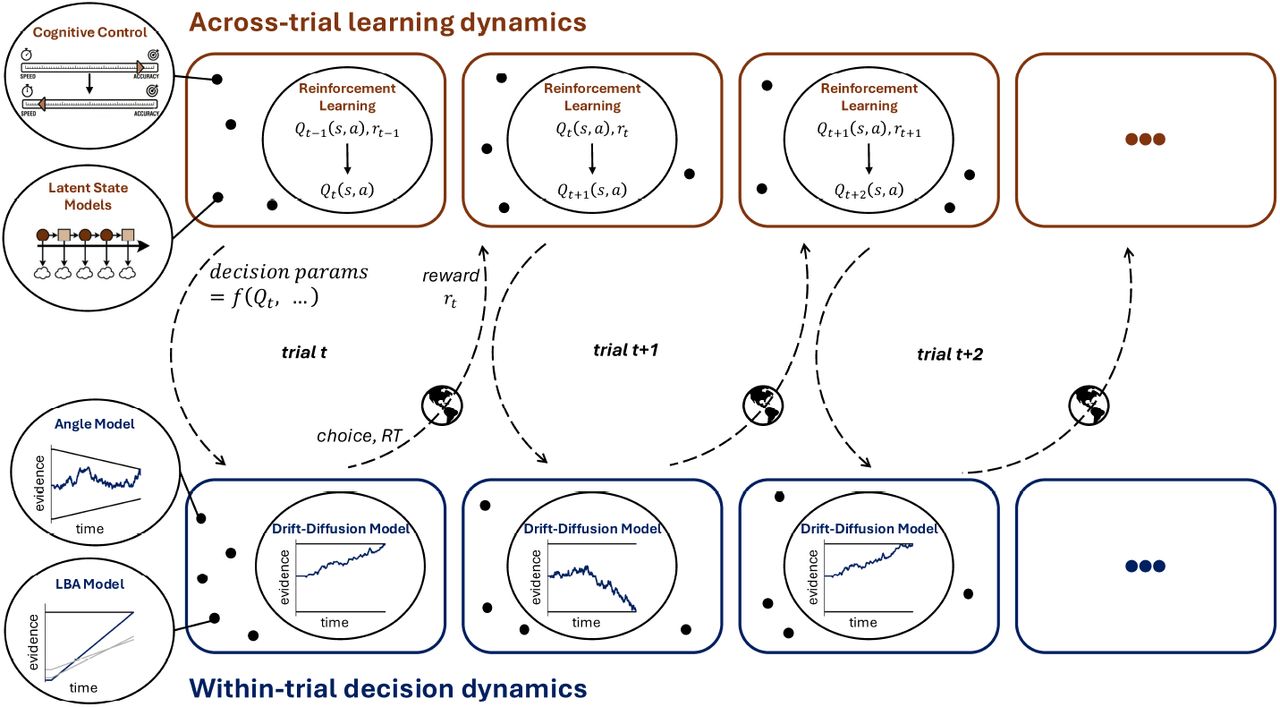
Figure reproduced from Fengler et al. (2026), "HSSM: A Widely Applicable Toolbox for Hierarchical Bayesian Neurocognitive Modeling". Article: https://doi.org/10.64898/2026.06.05.730398.

The exact notation in the paper is more detailed than we need here, but the core idea is the same as ssms.rl: a learning state informs a decision process parameter, and the resulting action/feedback pair determines the next learning state. A broader review of why RL and SSMs are complementary is Miletić, Boag, and Forstmann (2020): https://doi.org/10.1016/j.neuropsychologia.2019.107261.

The interleaved simulation loop¶

Because the parameters change with experience, RLSSM simulation is not a single fixed-parameter draw. It is an interleaved loop, repeated for every trial:

1. Start from the current learning state. In this tutorial that state is two Q-values, Q[0] and Q[1], one for each bandit arm.
2. Compute the trial-wise decision parameters. The Rescorla-Wagner learner produces drift via v = (Q[1] - Q[0]) * scaler. The scaler parameter converts a value difference into the numerical scale used by the decision process.
3. Simulate one SSM trial. The angle model uses drift plus fixed SSM parameters (a, z, t, theta) to generate a response and RT.
4. Map response to learning choice. The public response labels here are -1 and 1, but the learning rule updates zero-based choices 0 and 1.
5. Get context from the task environment. The selected bandit arm returns a feedback value such as 0 or 1. Other tasks could also provide fields such as condition, block, or stimulus_id.
6. Update the learning state. The prediction error is feedback - Q[choice]; the learning rate rl_alpha controls how strongly that error changes the selected Q-value.
7. Repeat with the new Q-values on the next trial.

One subtlety worth remembering: on each trial the drift is computed before the value update for that trial. This ordering matches HSSM's inference-side computation, which keeps simulation and inference consistent.

Where this fits in the HSSM ecosystem¶

Two packages work as a pair:

• ssm-simulators (this tutorial) — simulates synthetic RLSSM behavioral data.
• HSSM — performs Bayesian inference, recovering parameters from such data.

So a typical workflow is: design a model and simulate data with ssms.rl, then hand that data and model off to HSSM to fit it. Simulation is useful even before you have empirical data: it lets you check whether the model behaves as expected, whether plots show the learning pattern you intended, and whether HSSM can recover known parameters from generated data. We end the tutorial by showing the handoff surface.

1. Setup¶

Everything we need lives under a single import. The convention is to alias the namespace as rl. We also use pandas and matplotlib only for table inspection and plots; they are not part of the simulator API.

In [1]:

import ssms.rl as rl

import numpy as np
import pandas as pd
import matplotlib.pyplot as plt

import ssms.rl as rl import numpy as np import pandas as pd import matplotlib.pyplot as plt

2. The fastest path: presets¶

The quickest way to get going is a preset — a ready-made, validated model. A preset is useful when you want to focus on learning the workflow before deciding every model component yourself. The preset registry lets you discover what is available, inspect a model's "spec card", and fetch a configuration to simulate from.

In [2]:

# Which presets ship with the package?
rl.preset.list()

# Which presets ship with the package? rl.preset.list()

Out[2]:

['2AB_RW_Angle']

Each preset has readable metadata. Printing preset.info(...) gives you a compact "spec card": the task, the learning and decision processes, the parameters the model needs, sensible defaults, and the response labels it emits.

In [3]:

print(rl.preset.info("2AB_RW_Angle"))

print(rl.preset.info("2AB_RW_Angle"))

Preset: 2AB_RW_Angle
Description: Two-armed bandit with a Rescorla-Wagner delta-rule learner and an angle decision process.
Task: two-armed Bernoulli bandit
Learning process: RescorlaWagnerDrift
Decision process: angle
Required parameters: rl_alpha, scaler, a, z, t, theta
Default parameters: rl_alpha=0.2, scaler=2, a=1, z=0.5, t=0.001, theta=0
Response labels: (-1, 1)
Response to choice: {-1: 0, 1: 1}
Context fields: ['feedback']
Learning backend: jax
Gradient support: available
HSSM participant contract: yes

Reading the card top to bottom: 2AB_RW_Angle is a 2-Armed Bandit with a Rescorla–Wagner learner and an Angle decision process. It needs six parameters — two for learning (rl_alpha, scaler) and four for the angle SSM (a, z, t, theta) — and it emits responses labeled -1 and 1.

Now fetch the configuration and build a simulator from it. The configuration describes the model's structure; the actual parameter values are supplied separately as theta when we call simulate().

In [4]:

config = rl.preset.get("2AB_RW_Angle")
sim = rl.Simulator(config)

# Concrete parameter values for this run.
theta = {
    "rl_alpha": 0.3,  # learning rate
    "scaler": 2.0,    # maps learned value difference -> drift
    "a": 1.5,         # boundary separation (angle SSM)
    "z": 0.5,         # starting point
    "t": 0.3,         # non-decision time
    "theta": 0.2,     # boundary angle
}

data = sim.simulate(
    theta=theta,
    n_trials=120,
    n_participants=40,
    random_state=42,
)

data.head()

config = rl.preset.get("2AB_RW_Angle") sim = rl.Simulator(config) # Concrete parameter values for this run. theta = { "rl_alpha": 0.3, # learning rate "scaler": 2.0, # maps learned value difference -> drift "a": 1.5, # boundary separation (angle SSM) "z": 0.5, # starting point "t": 0.3, # non-decision time "theta": 0.2, # boundary angle } data = sim.simulate( theta=theta, n_trials=120, n_participants=40, random_state=42, ) data.head()

Out[4]:

	participant_id	trial_id	rt	response	feedback
0	0	0	2.999996	1	0.0
1	0	1	1.506524	-1	0.0
2	0	2	1.080149	-1	0.0
3	0	3	1.355910	-1	1.0
4	0	4	1.051847	-1	0.0

The result is a tidy "long" DataFrame — one row per trial — ready for analysis or inference. Its columns are:

• participant_id — which simulated participant (subject) the trial belongs to.
• trial_id — trial index within that participant, starting at 0.
• rt — the simulated response time, in seconds.
• response — the choice, using the model's response labels (-1 or 1 here).
• feedback — the task context field used by the learner for reward feedback.

Every participant has the same number of trials, in trial order: a balanced panel. That balanced, participant-contiguous layout is the shape downstream HSSM inference expects for the current RLSSM path. trial_id is ordinary useful data; the actual learning replay follows row order within each participant.

3. Model anatomy: the three pillars¶

The preset we just used is an ordinary configuration object. Looking inside it makes the three-pillar structure concrete — and shows where each parameter comes from. This is a useful habit: before simulating or fitting a model, inspect which part of the model owns each parameter.

In [5]:

print("Decision process    :", config.decision_process)
print("Learning process    :", type(config.learning_process).__name__)
print("Task environment    :", type(config.task_environment).__name__)
print("Computed SSM params :", config.learning_process.computed_params)
print("Context fields      :", config.context_fields)
print("Response -> choice  :", config.response_to_choice)
print("Free theta params   :", config.list_params)

print("Decision process :", config.decision_process) print("Learning process :", type(config.learning_process).__name__) print("Task environment :", type(config.task_environment).__name__) print("Computed SSM params :", config.learning_process.computed_params) print("Context fields :", config.context_fields) print("Response -> choice :", config.response_to_choice) print("Free theta params :", config.list_params)

Decision process    : angle
Learning process    : RescorlaWagnerDrift
Task environment    : Bandit
Computed SSM params : ['v']
Context fields      : ['feedback']
Response -> choice  : {-1: 0, 1: 1}
Free theta params   : ['rl_alpha', 'scaler', 'a', 'z', 't', 'theta']

The free parameter list is the learning parameters followed by the fixed SSM parameters:

• rl_alpha controls how strongly feedback changes the selected Q-value.
• scaler converts the learned value difference into drift rate.
• a, z, t, theta configure the angle SSM and stay fixed across trials.

The trial-wise drift v is not in theta, because it is computed by the learning process on every trial. That is the key handshake: learned state supplies the changing SSM parameter, while theta supplies the model parameters that are fixed for a participant or group.

4. Build a simple model yourself¶

Presets are just pre-assembled configurations — you can build the same thing by hand from the three pillars. Here we compose a Rescorla-Wagner learner, a Bernoulli bandit, and the angle decision process into a ModelConfig.

RescorlaWagnerDrift is the decision-facing Rescorla-Wagner class for two-action SSMs that need trial-wise drift v. The base RescorlaWagnerDeltaRule owns only the Q-value update; RescorlaWagnerSoftmax emits q0..qN for choice-only softmax decision processes.

A Bernoulli bandit is a task where each arm pays out a binary reward with a fixed probability. In the example below, arm 0 is better (0.7) than arm 1 (0.3), so a successful learner should gradually favor arm 0.

In [6]:

learner = rl.learning.RescorlaWagnerDrift(n_actions=2, initial_q=0.5)

task = rl.env.Bandit.bernoulli(
    probabilities=[0.7, 0.3],   # arm 0 pays off 70% of the time, arm 1 30%
    response_labels=[-1, 1],    # SSM emits -1 for arm 0, +1 for arm 1
)

my_config = rl.ModelConfig(
    model_name="my_first_rlssm",
    description="Rescorla-Wagner learner + Bernoulli bandit + angle SSM",
    decision_process="angle",
    learning_process=learner,
    task_environment=task,
)

my_config.list_params

learner = rl.learning.RescorlaWagnerDrift(n_actions=2, initial_q=0.5) task = rl.env.Bandit.bernoulli( probabilities=[0.7, 0.3], # arm 0 pays off 70% of the time, arm 1 30% response_labels=[-1, 1], # SSM emits -1 for arm 0, +1 for arm 1 ) my_config = rl.ModelConfig( model_name="my_first_rlssm", description="Rescorla-Wagner learner + Bernoulli bandit + angle SSM", decision_process="angle", learning_process=learner, task_environment=task, ) my_config.list_params

Out[6]:

['rl_alpha', 'scaler', 'a', 'z', 't', 'theta']

Notice we never spelled out the parameter list, bounds, or defaults — ModelConfig derived them automatically from the learning rule and the chosen SSM. Simulating from our hand-built model works exactly like the preset.

In [7]:

my_sim = rl.Simulator(my_config)
my_data = my_sim.simulate(theta=theta, n_trials=120, n_participants=40, random_state=7)
my_data.head()

my_sim = rl.Simulator(my_config) my_data = my_sim.simulate(theta=theta, n_trials=120, n_participants=40, random_state=7) my_data.head()

Out[7]:

	participant_id	trial_id	rt	response	feedback
0	0	0	1.172805	1	1.0
1	0	1	1.406510	1	0.0
2	0	2	2.123800	-1	0.0
3	0	3	0.979096	1	1.0
4	0	4	1.012957	1	0.0

Advanced tutorial: other learning rules (e.g. dual-learning-rate Rescorla–Wagner), Gaussian-reward bandits, the TaskConfig shorthand, and writing your own learning process or task environment.

5. Simulating multiple participants¶

We have already simulated 40 participants. By default, every participant shares the same theta, and you control the panel size with n_participants and n_trials. This is useful for a first simulation because it isolates stochastic variation: people can differ in their realized choices and RTs even when their generating parameters are identical.

In [8]:

small = sim.simulate(theta=theta, n_trials=10, n_participants=3, random_state=0)
small.groupby("participant_id").size()

small = sim.simulate(theta=theta, n_trials=10, n_participants=3, random_state=0) small.groupby("participant_id").size()

Out[8]:

participant_id
0    10
1    10
2    10
dtype: int64

Often you want participants to differ — for example, each with their own learning rate. You can pass a list for any parameter, with one value per participant; the simulator then infers the number of participants from that list.

In [9]:

theta_varying = {**theta, "rl_alpha": [0.1, 0.3, 0.6]}  # three participants
varied = sim.simulate(theta=theta_varying, n_trials=50, random_state=1)
sorted(varied["participant_id"].unique())

theta_varying = {**theta, "rl_alpha": [0.1, 0.3, 0.6]} # three participants varied = sim.simulate(theta=theta_varying, n_trials=50, random_state=1) sorted(varied["participant_id"].unique())

Out[9]:

[np.int64(0), np.int64(1), np.int64(2)]

Advanced tutorial: the full rules for participant-wise parameters — mixing scalar and list values, length checks, and how n_participants must agree with the lists.

6. Inspecting and visualizing the data¶

A simulated dataset is just a DataFrame, so the usual pandas + matplotlib tools apply. Three quick views tell us a lot about RLSSM data: a learning curve, a Q-value / drift replay, and the RT distribution.

Because arm 0 (response label -1) is the higher-reward option, a learner should choose -1 more and more often as trials progress.

In [10]:

# Proportion choosing the higher-reward option (response == -1), averaged across
# participants at each trial.
data = data.copy()
data["chose_high_reward"] = (data["response"] == -1).astype(float)
learning_curve = data.groupby("trial_id")["chose_high_reward"].mean()

fig, ax = plt.subplots(figsize=(7, 4))
ax.plot(learning_curve.index, learning_curve.values, color="C0")
ax.axhline(0.5, ls="--", color="gray", lw=1, label="chance")
ax.set_xlabel("Trial")
ax.set_ylabel("P(choose higher-reward option)")
ax.set_title("Learning curve (averaged over participants)")
ax.set_ylim(0, 1)
ax.legend()
plt.tight_layout()
plt.show()

# Proportion choosing the higher-reward option (response == -1), averaged across # participants at each trial. data = data.copy() data["chose_high_reward"] = (data["response"] == -1).astype(float) learning_curve = data.groupby("trial_id")["chose_high_reward"].mean() fig, ax = plt.subplots(figsize=(7, 4)) ax.plot(learning_curve.index, learning_curve.values, color="C0") ax.axhline(0.5, ls="--", color="gray", lw=1, label="chance") ax.set_xlabel("Trial") ax.set_ylabel("P(choose higher-reward option)") ax.set_title("Learning curve (averaged over participants)") ax.set_ylim(0, 1) ax.legend() plt.tight_layout() plt.show()

The curve climbs well above chance — the agents are learning. But the learning curve only shows choices. To see the RLSSM connection more directly, we can replay one participant's history and compute the hidden Q-value difference and drift rate used on each trial.

In [11]:

participant_history = data.loc[data["participant_id"] == 0, ["trial_id", "response", "feedback"]].reset_index(drop=True)

replay_learner = rl.learning.RescorlaWagnerDrift(n_actions=2, initial_q=0.5)
replay_state = replay_learner.init_state()
rl_params = {"rl_alpha": theta["rl_alpha"], "scaler": theta["scaler"]}

trajectory_rows = []
for trial in participant_history.itertuples(index=False):
    choice = config.response_to_choice[int(trial.response)]
    context = {
        "response": int(trial.response),
        "choice": choice,
        "feedback": float(trial.feedback),
    }
    computed = replay_learner.compute_python(replay_state, rl_params, context)
    q_values = replay_state["q_values"].copy()

    trajectory_rows.append(
        {
            "trial_id": int(trial.trial_id),
            "q_0": q_values[0],
            "q_1": q_values[1],
            "q_diff": q_values[1] - q_values[0],
            "drift": computed["v"],
            "response": int(trial.response),
            "feedback": float(trial.feedback),
            "choice": choice,
        }
    )
    replay_state = replay_learner.update_python(replay_state, rl_params, context)

trajectory = pd.DataFrame(trajectory_rows)

fig, axes = plt.subplots(2, 1, figsize=(8, 6), sharex=True)

axes[0].plot(trajectory["trial_id"], trajectory["q_diff"], color="C2")
axes[0].axhline(0, ls="--", color="gray", lw=1)
axes[0].set_ylabel("Q[1] - Q[0]")
axes[0].set_title("Learning state before each trial (participant 0)")

axes[1].plot(trajectory["trial_id"], trajectory["drift"], color="C3")
axes[1].axhline(0, ls="--", color="gray", lw=1)
axes[1].set_xlabel("Trial")
axes[1].set_ylabel("Drift rate v")
axes[1].set_title("Decision-process drift computed from the same values")

plt.tight_layout()
plt.show()

participant_history = data.loc[data["participant_id"] == 0, ["trial_id", "response", "feedback"]].reset_index(drop=True) replay_learner = rl.learning.RescorlaWagnerDrift(n_actions=2, initial_q=0.5) replay_state = replay_learner.init_state() rl_params = {"rl_alpha": theta["rl_alpha"], "scaler": theta["scaler"]} trajectory_rows = [] for trial in participant_history.itertuples(index=False): choice = config.response_to_choice[int(trial.response)] context = { "response": int(trial.response), "choice": choice, "feedback": float(trial.feedback), } computed = replay_learner.compute_python(replay_state, rl_params, context) q_values = replay_state["q_values"].copy() trajectory_rows.append( { "trial_id": int(trial.trial_id), "q_0": q_values[0], "q_1": q_values[1], "q_diff": q_values[1] - q_values[0], "drift": computed["v"], "response": int(trial.response), "feedback": float(trial.feedback), "choice": choice, } ) replay_state = replay_learner.update_python(replay_state, rl_params, context) trajectory = pd.DataFrame(trajectory_rows) fig, axes = plt.subplots(2, 1, figsize=(8, 6), sharex=True) axes[0].plot(trajectory["trial_id"], trajectory["q_diff"], color="C2") axes[0].axhline(0, ls="--", color="gray", lw=1) axes[0].set_ylabel("Q[1] - Q[0]") axes[0].set_title("Learning state before each trial (participant 0)") axes[1].plot(trajectory["trial_id"], trajectory["drift"], color="C3") axes[1].axhline(0, ls="--", color="gray", lw=1) axes[1].set_xlabel("Trial") axes[1].set_ylabel("Drift rate v") axes[1].set_title("Decision-process drift computed from the same values") plt.tight_layout() plt.show()

The two panels have the same shape because this model uses a simple link:

v = (Q[1] - Q[0]) * scaler

That link is the bridge between the learning process and the decision process. The learning rule does not directly choose for the agent; instead, it changes the drift rate that the SSM uses to generate a choice and RT. When Q[1] - Q[0] is negative, drift favors the response associated with arm 0 (-1 here). When it is positive, drift favors arm 1 (1).

Next, we look at the RT distribution, split by which option was chosen.

In [12]:

fig, ax = plt.subplots(figsize=(7, 4))
for label, color in [(-1, "C0"), (1, "C1")]:
    rts = data.loc[data["response"] == label, "rt"]
    ax.hist(rts, bins=40, alpha=0.6, color=color, label=f"response = {label}")
ax.set_xlabel("Response time (s)")
ax.set_ylabel("Count")
ax.set_title("RT distribution by choice")
ax.legend()
plt.tight_layout()
plt.show()

fig, ax = plt.subplots(figsize=(7, 4)) for label, color in [(-1, "C0"), (1, "C1")]: rts = data.loc[data["response"] == label, "rt"] ax.hist(rts, bins=40, alpha=0.6, color=color, label=f"response = {label}") ax.set_xlabel("Response time (s)") ax.set_ylabel("Count") ax.set_title("RT distribution by choice") ax.legend() plt.tight_layout() plt.show()

7. From simulation to inference¶

The point of simulating data is usually to test inference — can a model recover the parameters that generated the data? That is HSSM's job. Two small steps connect the two packages: validating the data, and handing it off.

Validation is worth doing even for simulated data because it catches mismatches that are easy to miss: a renamed feedback column, invalid response labels, missing RTs, or rows that are no longer ordered by participant and trial.

Validate the data¶

Before inference, it helps to check that a dataset has the structure HSSM expects (required columns, a balanced and trial-ordered panel, valid response labels, no stray missing values). config.validate_data(...) does this and returns a report you can print, or turn into an error if something is wrong.

In [13]:

report = config.validate_data(data)
report.print()

# In a script you would typically guard with:
#   report.raise_for_errors()   # raises if the data is not inference-ready

report = config.validate_data(data) report.print() # In a script you would typically guard with: # report.raise_for_errors() # raises if the data is not inference-ready

RLSSM data validation report:
  [WARNING] extra_columns: data has extra columns not required by this model: ['chose_high_reward', 'trial_id'].
  panel shape: participants=40, trials_per_participant=120

Hand off to HSSM¶

HSSM consumes an ssms.rl model through a small bridge. The simulator side exposes the model's structure as a plain dictionary, which is a useful thing to inspect. In the Milestone 4 contract, observable task/design columns are called context_fields, and the participant contract shows the exact participant-history columns used to replay learning during inference:

In [14]:

bridge_dict = config.to_hssm_config_dict()

print("model_name      :", bridge_dict["model_name"])
print("decision_process:", bridge_dict["decision_process"])
print("list_params     :", bridge_dict["list_params"])
print("context_fields  :", bridge_dict["context_fields"])
print("computed_outputs:", bridge_dict["participant_contract"]["computed_outputs"])
print("input_fields    :", bridge_dict["participant_contract"]["input_fields"])

bridge_dict = config.to_hssm_config_dict() print("model_name :", bridge_dict["model_name"]) print("decision_process:", bridge_dict["decision_process"]) print("list_params :", bridge_dict["list_params"]) print("context_fields :", bridge_dict["context_fields"]) print("computed_outputs:", bridge_dict["participant_contract"]["computed_outputs"]) print("input_fields :", bridge_dict["participant_contract"]["input_fields"])

model_name      : 2AB_RW_Angle
decision_process: angle
list_params     : ['rl_alpha', 'scaler', 'a', 'z', 't', 'theta']
context_fields  : ['feedback']
computed_outputs: ['v']
input_fields    : ['rl_alpha', 'scaler', 'response', 'feedback']

On the HSSM side, you don't assemble any of this by hand. HSSM provides a factory that takes the ssms.rl model (by preset name or config object), assembles the simulator-side participant function with the JAX backend, and builds a ready-to-fit HSSM config. The code below is illustrative — it requires HSSM to be installed and is not run as part of this simulator tutorial:

import hssm

# Build an HSSM model directly from the ssms.rl model.
hssm_config = hssm.rl.RLSSMConfig.from_ssms_model(config)   # or "2AB_RW_Angle"
model = hssm.RLSSM(data=data, model_config=hssm_config)

# ... then sample and inspect as usual:
# idata = model.sample()

Internally, HSSM carries ssms.rl context_fields through its RLSSM data-column plumbing and uses the assembled participant function to compute every trial-wise SSM parameter declared by the simulator model. A higher-level constructor — hssm.RLSSM(data, model="2AB_RW_Angle") — is planned but not yet available, so for now use RLSSMConfig.from_ssms_model(...). For the full end-to-end inference and parameter-recovery workflow, see the ssms.rl API reference.

8. Summary and next steps¶

You now know the whole basic arc:

• An RLSSM = a learning process + a decision process (SSM) + a task environment, simulated in an interleaved trial-by-trial loop.
• The learning process updates Q-values from feedback; the decision process turns the current value state into choice and RT.
• In the preset model, Q[1] - Q[0] is scaled into the trial-wise drift rate v, which is why plotting Q-value differences and drift helps diagnose whether learning is informing the decision process as intended.
• More general ssms.rl models can compute other trial-wise decision parameters too; the advanced tutorial shows that handshake explicitly.
• Presets (rl.preset.list / info / get) are the fastest way to a working model.
• A ModelConfig can be built by hand from the three pillars; rl.Simulator turns it (plus a theta of parameter values) into a balanced panel of behavioral data, for one or many participants.
• The data is a tidy DataFrame you can inspect, plot, validate, and hand off to HSSM for inference.

Other useful beginner exercises:

• Change rl_alpha and watch how quickly the learning curve moves away from chance.
• Change scaler and watch how strongly the same Q-value difference affects drift and RTs.
• Simulate a few participant-wise rl_alpha values and compare their learning curves.
• Use config.validate_data(...) on a deliberately edited dataset to see the repair hints.

Continue with the advanced tutorial, which covers:

• response labels vs. zero-based learning choices, and explicit response_to_choice;
• alternative components: dual-learning-rate Rescorla-Wagner, Gaussian-reward bandits, the TaskConfig shorthand, and custom task/learning components;
• context-aware learning with task/design columns such as condition;
• full participant-wise theta rules;
• posterior predictive simulation with mode="ppc";
• validation failure modes;
• assembled models, multi-output computed parameters, and the HSSM bridge internals.