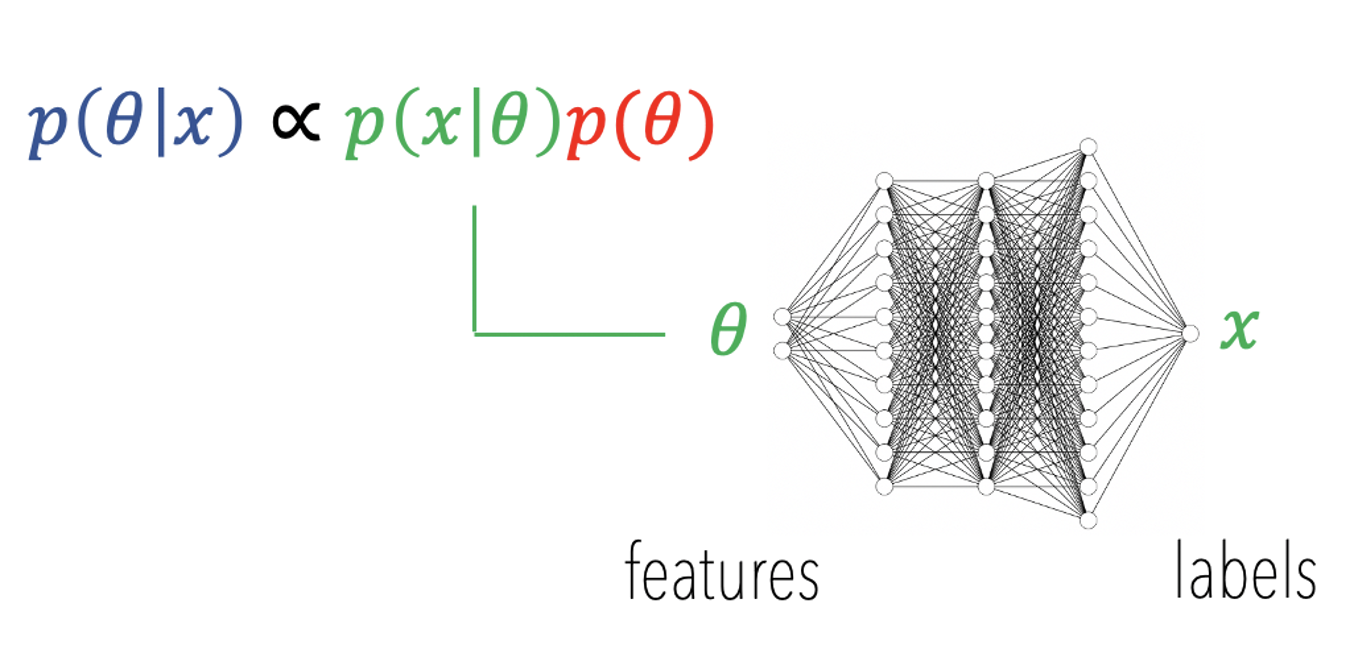
HSSM MathPsych 2025¶

Welcome to the PyMC to HSSM tutorial:

This is an advanced tutorial, taught as part of a workshop session during the conference for Mathematical Psychology, held in Columbus Ohio, 2025.

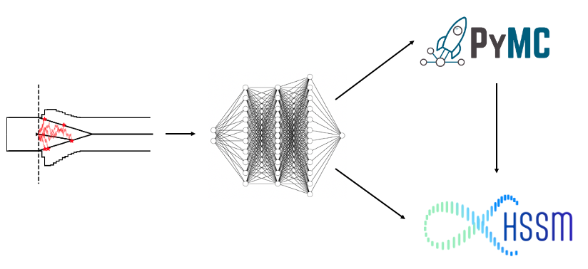
In this short tutorial we will explore some of the features of HSSM that are geared towards users who want to do one of three things:

1. Build custom PyMC models around observation models build via HSSM low-level utilities (to e.g. break out of the hierarchical regression corsett imposed via the Bambi interface)
2. Work with custom models that are not provided by HSSM out of the box via the High-Level Interface (please consider contributing directly to the HSSM ecosystem eventually :))
3. Break our of PyMC/HSSM on the tail end to apply your own samplers!

Colab Instructions¶

If you would like to run this tutorial on Google colab, please click this link.

Once you are in the colab:

1. Follow the installation instructions below (uncomment the respective code)
2. restart your runtime.

NOTE:

You may want to switch your runtime to have a GPU or TPU. To do so, go to Runtime > Change runtime type and select the desired hardware accelerator. Note that if you switch your runtime you have to follow the installation instructions again.

In [1]:

# If running this on Colab, please uncomment the next line
# !pip install hssm
# !pip install onnxruntime
# !pip install "zeus-mcmc>=2.5.4"

# If running this on Colab, please uncomment the next line # !pip install hssm # !pip install onnxruntime # !pip install "zeus-mcmc>=2.5.4"

In [2]:

# # Data Files
# !wget -P  data/mathpsych_workshop_2025_data https://raw.githubusercontent.com/lnccbrown/HSSM/main/docs/tutorials/pymc_to_hssm/mathpsych_workshop_2025_data/race_3_no_bias_lan_batch.onnx
# !wget -P  data/mathpsych_workshop_2025_data https://raw.githubusercontent.com/lnccbrown/HSSM/main/docs/tutorials/pymc_to_hssm/mathpsych_workshop_2025_data/ddm_lan_batch.onnx

# # Data Files # !wget -P data/mathpsych_workshop_2025_data https://raw.githubusercontent.com/lnccbrown/HSSM/main/docs/tutorials/pymc_to_hssm/mathpsych_workshop_2025_data/race_3_no_bias_lan_batch.onnx # !wget -P data/mathpsych_workshop_2025_data https://raw.githubusercontent.com/lnccbrown/HSSM/main/docs/tutorials/pymc_to_hssm/mathpsych_workshop_2025_data/ddm_lan_batch.onnx

Start of Tutorial¶

Load Modules¶

In [3]:

import os
from pathlib import Path
from copy import deepcopy
import matplotlib.pyplot as plt
import numpy as np

import hssm
import ssms
import arviz as az

import onnx
import onnxruntime as ort

import os from pathlib import Path from copy import deepcopy import matplotlib.pyplot as plt import numpy as np import hssm import ssms import arviz as az import onnx import onnxruntime as ort

Getting ourselves a LAN / Likelihood-Network¶

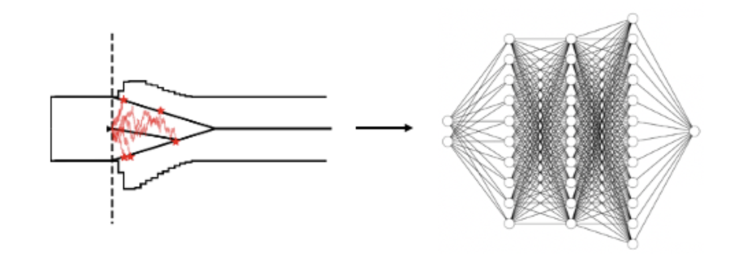
As you will see over the course of this tutorial, ultimately we don't care about where networks might come from. Here we rely on our own pipeline to train a LAN, however the conceptual part of this tutorial translates to likelihood functions that are derived from really any source, such as e.g. coming directly out of the BayesFlow package.

Our pipeline relies on two support packages:

1. ssm-simulators: A package with focus on fast simulation of sequential sampling models
2. LanFactory: A package to train simple neural networks geared to work seemlessly with training data generated from ssm-simulators

ssm-simulators is designed to be simple to contribute to (we continuously improve that aspect), so if you design new simulators, you should find it quite easy to add them to the package.

Training Data¶

Once you have your simulator implemented, you can specify a simple .yaml file, with a variation of the following contents:

MODEL: 'race_3_no_bias'
N_SAMPLES: 2000
N_PARAMETER_SETS: 100
DELTA_T: 0.001
N_TRAINING_SAMPLES_BY_PARAMETER_SET: 200
N_SUBRUNS: 20
GENERATOR_APPROACH: 'lan'

You can use the following command to generate training data:

generate --config-path <path/to/config.yaml> \
         --output <output/directory>

(Please see the basic Readme for a more complete explanation)

Network Training¶

Once we have our training data, we can again use a single command to train the network. We only need to specify a few network features in a network_config.yaml file and train

NETWORK_TYPE: "lan" 
CPU_BATCH_SIZE: 1000
N_EPOCHS: 20
MODEL: "ddm"
LAYER_SIZES: [[100, 100, 100, 1]]
ACTIVATIONS: [['tanh', 'tanh', 'tanh']]
LABELS_LOWER_BOUND: np.log(1e-7)

Now we simply call:

torchtrain --config-path <path/to/network_config.yaml> \
           --training-data-folder <path/to/training-data> \
           --dl-workers 3 \
           --network-path-base <my_trained_network>`

(Same thing, this is explained in the baseid Readme on the github page of the package)

In [4]:

# !torchtrain --config-path pymc_to_hssm/network_config.yaml --training-data-folder torch_nb_data/training_data --dl-workers 4 --networks-path-base pymc_to_hssm/example_network/

# !torchtrain --config-path pymc_to_hssm/network_config.yaml --training-data-folder torch_nb_data/training_data --dl-workers 4 --networks-path-base pymc_to_hssm/example_network/

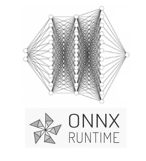
Working Directly with .onnx networks¶

Utilities¶

The below utility turns a network which may be defined for single datapoints into a batchable version of itself (so that call can work in parallel over the trial-dimension). We assume below that all our networks are already batchable, but keep this utility here for your convenience.

In [5]:

def make_batchable(onnx_model,
                   folder_path = "pymc_to_hssm/mathpsych_2025_data",
                   file_name = "ddm_lan_batch.onnx"):

    # Change input and output dimensions to be dynamic to allow for batching
    # (in case this is not already done)
    
    for input_tensor in onnx_model.graph.input:
        dim_proto = input_tensor.type.tensor_type.shape.dim[0]
        if not dim_proto.dim_param == "None":
            dim_proto.dim_param = "None"

    for output_tensor in onnx_model.graph.output:
        dim_proto = output_tensor.type.tensor_type.shape.dim[0]
        if not dim_proto.dim_param == "None":
            dim_proto.dim_param = "None"
    os.makedirs(folder_path, exist_ok = True)
    onnx.save(onnx_model, Path(folder_path, file_name))

def make_batchable(onnx_model, folder_path = "pymc_to_hssm/mathpsych_2025_data", file_name = "ddm_lan_batch.onnx"): # Change input and output dimensions to be dynamic to allow for batching # (in case this is not already done) for input_tensor in onnx_model.graph.input: dim_proto = input_tensor.type.tensor_type.shape.dim[0] if not dim_proto.dim_param == "None": dim_proto.dim_param = "None" for output_tensor in onnx_model.graph.output: dim_proto = output_tensor.type.tensor_type.shape.dim[0] if not dim_proto.dim_param == "None": dim_proto.dim_param = "None" os.makedirs(folder_path, exist_ok = True) onnx.save(onnx_model, Path(folder_path, file_name))

Network Path¶

In [6]:

ddm_network_path = Path("pymc_to_hssm",
                        "mathpsych_workshop_2025_data",
                        "ddm_lan_batch.onnx")

ddm_network_path = Path("pymc_to_hssm", "mathpsych_workshop_2025_data", "ddm_lan_batch.onnx")

Load and time Network¶

We will work natively with with neural networks that are encoded as .onnx files. In this part , but here we first focus on loading an .onnx file into an onnx runtime, just to give an idea what .onnx is about.

Below we load a network, and time the forward pass, which should translate to the evaluation time we can expect for a single likelihood. We will illustrate this approach a bit later.

In [7]:

# Load onnx model
onnx_model = onnx.load(ddm_network_path)
input_name = onnx_model.graph.input[0].name
ort_session = ort.InferenceSession(onnx_model.SerializeToString())

# Test inference speed
import time

start = time.time()
for i in range(100):
    ort_session.run(
        None, {input_name: np.random.uniform(size=(1000, 6)).astype(np.float32)}
    )
end = time.time()
print(f"Time taken: {(end - start) / 100} seconds")

# Load onnx model onnx_model = onnx.load(ddm_network_path) input_name = onnx_model.graph.input[0].name ort_session = ort.InferenceSession(onnx_model.SerializeToString()) # Test inference speed import time start = time.time() for i in range(100): ort_session.run( None, {input_name: np.random.uniform(size=(1000, 6)).astype(np.float32)} ) end = time.time() print(f"Time taken: {(end - start) / 100} seconds")

Time taken: 0.0002436685562133789 seconds

HSSM: Low-level Interface¶

We will first work with .onnx files by directly refering to the filepath and letting our utilities take care of the rest. However, we will see one example at the end, where we manually construct a likelihood from an instantiated .onnx runtime.

Example (1): Construct your own random variable¶

Under the hood, a lot of the heavy lifting done by HSSM boils down to the creating of valid Random Variables that are compatible with PyMC specifications.

In broad strokes: In probabilist programming, a minimal specification for a random variable that let's us sample all the quantities of interest for a standard Bayesian Analysis are:

• A likelihood function
• A valid simulator

If we have both of these, we can do everything. We can sample from the posterior, from the prior predictive and from the posterior predictive,which will cover essentially 99.9% of our needs.

Below, we use HSSM low level functionality to construct such a random variable in three simple steps. Once constructed we use it in a PyMC model natively!

Note:

Truth be told, we can run MCMC without ever supplying a valid simulator and other tutorials showcase that scenario. However in such cases you are on your own once you want to sample from posterior predictives and/or prior predictives.

Model¶

Data¶

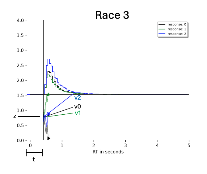
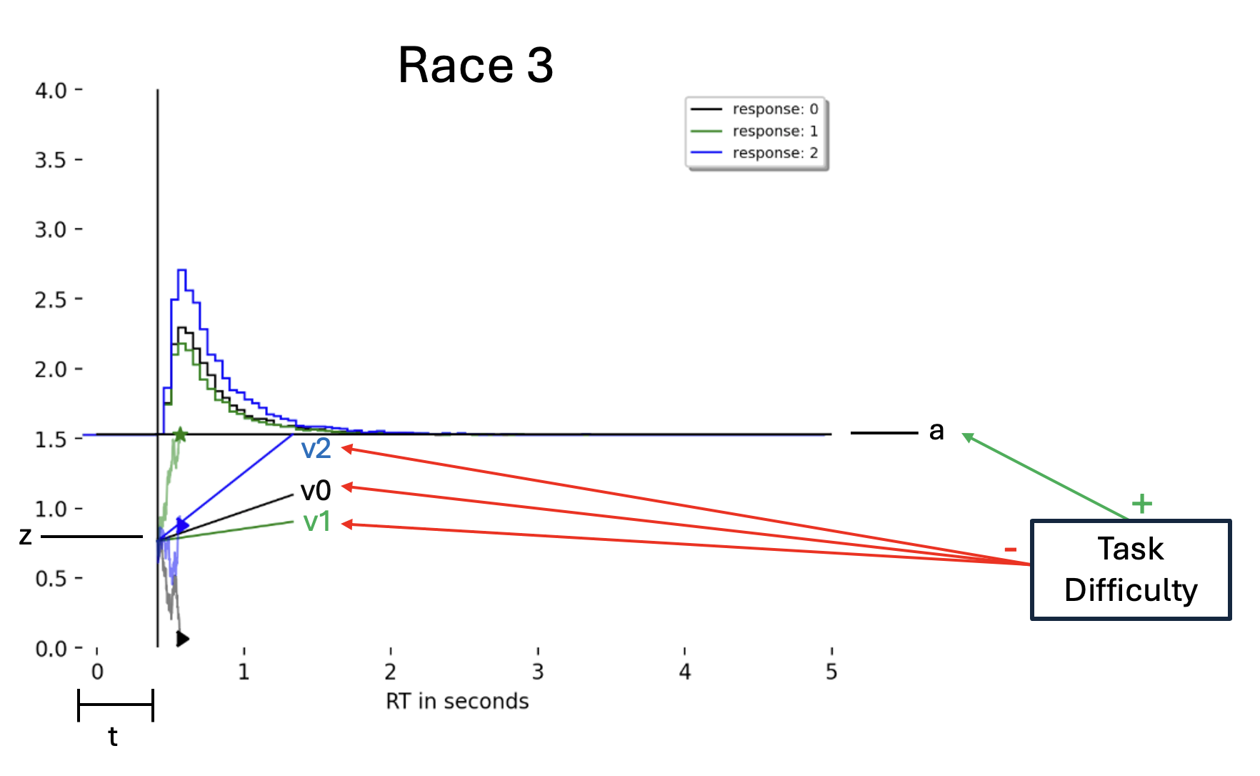
We simulate a simple dataset consisting fo $750$ trials from the Race 3 model as depicted above. HSSM has a simulate_data() function which comes in handy for this purpose. We can access all named models which are implemented in the ssm-simulators package.

In [8]:

# Set parameters
v0 = 1.5
v1 = 0.5
v2 = 0.5
a = 1.5
t = 0.3
z = 0.5

# simulate some data from the model
obs_race3 = hssm.simulate_data(
    theta=dict(v0=v0, v1=v1, v2=v2, a=a, t=t, z=z), model="race_no_bias_3", size=750
)

# Set parameters v0 = 1.5 v1 = 0.5 v2 = 0.5 a = 1.5 t = 0.3 z = 0.5 # simulate some data from the model obs_race3 = hssm.simulate_data( theta=dict(v0=v0, v1=v1, v2=v2, a=a, t=t, z=z), model="race_no_bias_3", size=750 )

Utilities¶

While we can use fully custom simulators in the context of this tutorial, we are sticking to simulators implemented in ssm-simulators ssm-simulators has model configuration dictionaries for every model that is implemented in the package.

Let's take a peak below, since we have to pass various elements of this dictionary to downstream utility functions.

In [9]:

ssms.config.model_config["race_no_bias_3"]

ssms.config.model_config["race_no_bias_3"]

Out[9]:

{'name': 'race_no_bias_3',
 'params': ['v0', 'v1', 'v2', 'a', 'z', 't'],
 'param_bounds': [[0.0, 0.0, 0.0, 1.0, 0.0, 0.0],
  [2.5, 2.5, 2.5, 3.0, 0.9, 2.0]],
 'boundary_name': 'constant',
 'boundary': <function ssms.basic_simulators.boundary_functions.constant(t: float | numpy.ndarray = 0) -> float | numpy.ndarray>,
 'n_params': 6,
 'n_particles': 3,
 'default_params': [0.0, 0.0, 0.0, 2.0, 0.5, 0.001],
 'nchoices': 3,
 'choices': [0, 1, 2],
 'simulator': <cyfunction race_model at 0x2ac625a80>}

In [10]:

race_3_model_config = deepcopy(ssms.config.model_config["race_no_bias_3"])

race_3_model_config = deepcopy(ssms.config.model_config["race_no_bias_3"])

In [11]:

# Little utilitiy to transform the list entry for parameter bounds into a dictionary
def make_param_bound_dict(config):
    param_bounds = config["param_bounds"]
    print(param_bounds)
    param_names = config['params']
    print(param_names)
    return {param_names[i]: (param_bounds[0][i],
                             param_bounds[1][i]) for i in range(len(param_names))}

# Little utilitiy to transform the list entry for parameter bounds into a dictionary def make_param_bound_dict(config): param_bounds = config["param_bounds"] print(param_bounds) param_names = config['params'] print(param_names) return {param_names[i]: (param_bounds[0][i], param_bounds[1][i]) for i in range(len(param_names))}

Setting the Network Path¶

In [12]:

# Networks
network_path = Path("pymc_to_hssm",
                    "mathpsych_workshop_2025_data",
                    "race_3_no_bias_lan_batch.onnx")

# Networks network_path = Path("pymc_to_hssm", "mathpsych_workshop_2025_data", "race_3_no_bias_lan_batch.onnx")

Networks to Random Variables¶

Remember that the .onnx file is just a representation for a neural network... this Network is actually a LAN, and hence, by definition differentiable with respect to it's inputs (the parameters of the model).

HSSM will help you construct costom PyMC random variables starting from .onnx files. We will see two routes to work with custom distributions in PYMC and HSSM, however more routes exist, and are in the making. Here is a list:

1. Any valid Python function (we will see this later): The blackbox regime
2. .onnx function with Network signature: approx_differentiable
3. JAX function with Network signature: appox_differentiable
4. PyTensor function / JAX function with valid likelihood signature: analytical

We will ow focus on route 2., directly through PyMC, using HSSM only as a help in constructing random variabels. We will then showcase how the HSSM high-level (main) interface still allows us to work with option 2. very conveniently.

Last, we are going to showcase option 1. via the HSSM high-level interface.

Constructing the Random Variable¶

To construct out PyMC random variables we make use of two utilities HSSM provides.

1. make_likelihood_callable() allows us to pass the network path, as well as a few configuration arguments, and will construct a valid callable likelihood function (duh..) for us
2. make_distribution() attaches a simulator (if it is part of the ssms-simulators package we can pass a string here) and assembles a valid PyMC distribution for us

In [13]:

from hssm.distribution_utils.dist import (
    make_distribution,
    make_likelihood_callable,
)

# Step 1: Define a likelihood function
logp_jax_op = make_likelihood_callable(
    loglik=network_path,
    loglik_kind="approx_differentiable",
    backend="jax",
    params_is_reg=[True for _ in range(len(race_3_model_config["params"]))],
    # params_only=False,
)

# Step 2: Define a distribution
CustomDistribution = make_distribution(
    rv="race_no_bias_3", # CustomRV,
    loglik=logp_jax_op,
    list_params=race_3_model_config["params"],
    bounds=make_param_bound_dict(race_3_model_config),
)

from hssm.distribution_utils.dist import ( make_distribution, make_likelihood_callable, ) # Step 1: Define a likelihood function logp_jax_op = make_likelihood_callable( loglik=network_path, loglik_kind="approx_differentiable", backend="jax", params_is_reg=[True for _ in range(len(race_3_model_config["params"]))], # params_only=False, ) # Step 2: Define a distribution CustomDistribution = make_distribution( rv="race_no_bias_3", # CustomRV, loglik=logp_jax_op, list_params=race_3_model_config["params"], bounds=make_param_bound_dict(race_3_model_config), )

[[0.0, 0.0, 0.0, 1.0, 0.0, 0.0], [2.5, 2.5, 2.5, 3.0, 0.9, 2.0]]
['v0', 'v1', 'v2', 'a', 'z', 't']

Note

make_likelihood_callable() has a parameter params_is_reg to which we pass a list of boolean variables (all set to True) in our case.

This argument sets parameters of our likelihood to scalars or vectors (trial-wise, is_reg for whether the parameter could be the outcome of a regression). For simplicity we set all parameters to vectors as a default.

The conseuqence is that we will define our PyMC model below with that expectation, and multiple all our parameters by a fixed vector of ones to establish the trial-wise relation.

First PyMC model¶

We could (and have) spend a whole workshop, or many, to introduce the basics of PyMC itself. It is a rich library, connects to a deep eco-system around probabilistic programming and allows us to construct generative models around our core SSM, in ways that allows us to test a plethora of hypothesis about a given dataset.

We will, however, not get distracted too much by the intricacies of PyMC, and instead just use this occasion to showcase that in general all doors are now open.

As a very basic principle, consider the construction of a PyMC model as:

1. Setting data (Data Block)
2. Defining priors over parameters (Priors Block)
3. Defining any kind of transformation on the parameters (Deterministics Block)
4. Defining our observation model that observes our data and ingests trial level transformed parameters (Likelihood Block)

In [14]:

import pymc as pm
import pytensor.tensor as pt


param_bounds_race_3 = make_param_bound_dict(race_3_model_config)

with pm.Model() as race3_pymc:
    # Data
    obs_pt = pm.Data("obs", obs_race3[["rt", "response"]].values)

    # Priors
    v0 = pm.Uniform("v0", 
                   lower=param_bounds_race_3["v0"][0],
                   upper=param_bounds_race_3["v0"][1],
                   initval=1.0)
    v1 = pm.Uniform("v1", 
                   lower=param_bounds_race_3["v1"][0],
                   upper=param_bounds_race_3["v1"][1],
                   initval=1.0)
    v2 = pm.Uniform("v2", 
                   lower=param_bounds_race_3["v2"][0],
                   upper=param_bounds_race_3["v2"][1],
                   initval=1.0)
    a = pm.Uniform("a",
                      lower=param_bounds_race_3["a"][0],
                      upper=param_bounds_race_3["a"][1],
                      initval=2.0)
    z = 0.5 # We fix this parameter because it is extremely hard to jointly identify both z and a
    t = pm.Uniform("t",
                   lower=param_bounds_race_3["t"][0],
                   upper=param_bounds_race_3["t"][1],
                   initval=0.1)

    # Vectorize parameters (Deterministics)
    v0_reg = pm.Deterministic("v0_reg", v0 * pt.ones_like(obs_race3.values[:, 0]))
    v1_reg = pm.Deterministic("v1_reg", v1 * pt.ones_like(obs_race3.values[:, 0]))
    v2_reg = pm.Deterministic("v2_reg", v2 * pt.ones_like(obs_race3.values[:, 0]))
    a_reg = pm.Deterministic("a_reg", a * pt.ones_like(obs_race3.values[:, 0]))
    t_reg = pm.Deterministic("t_reg", t * pt.ones_like(obs_race3.values[:, 0]))
    z_reg = pm.Deterministic("z_reg", z * pt.ones_like(obs_race3.values[:, 0]))

    # Likelihood
    race3_obs = CustomDistribution(
        "Race3", v0=v0_reg, v1=v1_reg, v2=v2_reg, a=a_reg, z=z_reg, t=t_reg, observed=obs_pt
    )

import pymc as pm import pytensor.tensor as pt param_bounds_race_3 = make_param_bound_dict(race_3_model_config) with pm.Model() as race3_pymc: # Data obs_pt = pm.Data("obs", obs_race3[["rt", "response"]].values) # Priors v0 = pm.Uniform("v0", lower=param_bounds_race_3["v0"][0], upper=param_bounds_race_3["v0"][1], initval=1.0) v1 = pm.Uniform("v1", lower=param_bounds_race_3["v1"][0], upper=param_bounds_race_3["v1"][1], initval=1.0) v2 = pm.Uniform("v2", lower=param_bounds_race_3["v2"][0], upper=param_bounds_race_3["v2"][1], initval=1.0) a = pm.Uniform("a", lower=param_bounds_race_3["a"][0], upper=param_bounds_race_3["a"][1], initval=2.0) z = 0.5 # We fix this parameter because it is extremely hard to jointly identify both z and a t = pm.Uniform("t", lower=param_bounds_race_3["t"][0], upper=param_bounds_race_3["t"][1], initval=0.1) # Vectorize parameters (Deterministics) v0_reg = pm.Deterministic("v0_reg", v0 * pt.ones_like(obs_race3.values[:, 0])) v1_reg = pm.Deterministic("v1_reg", v1 * pt.ones_like(obs_race3.values[:, 0])) v2_reg = pm.Deterministic("v2_reg", v2 * pt.ones_like(obs_race3.values[:, 0])) a_reg = pm.Deterministic("a_reg", a * pt.ones_like(obs_race3.values[:, 0])) t_reg = pm.Deterministic("t_reg", t * pt.ones_like(obs_race3.values[:, 0])) z_reg = pm.Deterministic("z_reg", z * pt.ones_like(obs_race3.values[:, 0])) # Likelihood race3_obs = CustomDistribution( "Race3", v0=v0_reg, v1=v1_reg, v2=v2_reg, a=a_reg, z=z_reg, t=t_reg, observed=obs_pt )

[[0.0, 0.0, 0.0, 1.0, 0.0, 0.0], [2.5, 2.5, 2.5, 3.0, 0.9, 2.0]]
['v0', 'v1', 'v2', 'a', 'z', 't']

String Representation of Model¶

In [15]:

race3_pymc

race3_pymc

Out[15]:

$$ \begin{array}{rcl} \text{v0} &\sim & \operatorname{Uniform}(0,~2.5)\\\text{v1} &\sim & \operatorname{Uniform}(0,~2.5)\\\text{v2} &\sim & \operatorname{Uniform}(0,~2.5)\\\text{a} &\sim & \operatorname{Uniform}(1,~3)\\\text{t} &\sim & \operatorname{Uniform}(0,~2)\\\text{v0\_reg} &\sim & \operatorname{Deterministic}(f(\text{v0}))\\\text{v1\_reg} &\sim & \operatorname{Deterministic}(f(\text{v1}))\\\text{v2\_reg} &\sim & \operatorname{Deterministic}(f(\text{v2}))\\\text{a\_reg} &\sim & \operatorname{Deterministic}(f(\text{a}))\\\text{t\_reg} &\sim & \operatorname{Deterministic}(f(\text{t}))\\\text{z\_reg} &\sim & \operatorname{Deterministic}(f())\\\text{Race3} &\sim & \operatorname{SSM}(\text{v0\_reg},~\text{v1\_reg},~\text{v2\_reg},~\text{a\_reg},~\text{z\_reg},~\text{t\_reg}) \end{array} $$

Graph Representation of Model¶

In [16]:

pm.model_to_graphviz(model=race3_pymc)

pm.model_to_graphviz(model=race3_pymc)

Out[16]:

Sample¶

In [17]:

with race3_pymc:
    # Sample Posterior
    race3_pymc_trace = pm.sample(nuts_sampler = "numpyro",
                                 chains = 2,
                                 tune = 500,
                                 draws = 500)
    # Get Posterior Predictive Samples
    pm.sample_posterior_predictive(race3_pymc_trace,
                                   extend_inferencedata=True)

with race3_pymc: # Sample Posterior race3_pymc_trace = pm.sample(nuts_sampler = "numpyro", chains = 2, tune = 500, draws = 500) # Get Posterior Predictive Samples pm.sample_posterior_predictive(race3_pymc_trace, extend_inferencedata=True)

  0%|          | 0/1000 [00:00<?, ?it/s]

  0%|          | 0/1000 [00:00<?, ?it/s]

We recommend running at least 4 chains for robust computation of convergence diagnostics
Sampling: [Race3]

Output()

Example (2): Slightly more complicate PyMC model¶

Once we are in the PyMC-universe directly, we can build models very flexibly. This includes

1. Introducing hierarchies
2. Complicated non-linear transformations on parameters
3. Time series approaches as processes over parameters (more on that by Krishn later)
4. and much much more!

Obviously this allows for things to go wrong, but you can have great fun along the way :)

Below we will build a model that is easy enough in principle, but specifically hard (impossible) to construct via the HSSM user interface directly. But more on that a bit later!

Simulate Data¶

Notice in the data simulation below: We are applying a regresion to all of v0, v1, v2 and a and de facto the beta parameter is shared amongst all four.

In [18]:

# Simple Regression Setup
beta = 0.5
difficulty = np.random.uniform(low = -1,
                               high = 1,
                               size = 750)

# Set parameters
v0 = 1.75 - beta * difficulty
v1 = 1.75 - beta * difficulty
v2 = 1.2 - beta * difficulty
a = 2.0 + beta * difficulty
t = 0.3
z = 0.5

# simulate some data from the model
obs_race3_reg = hssm.simulate_data(
    theta=dict(v0=v0, v1=v1, v2=v2, a=a, t=t, z=z), model="race_no_bias_3", size=1
)

# Simple Regression Setup beta = 0.5 difficulty = np.random.uniform(low = -1, high = 1, size = 750) # Set parameters v0 = 1.75 - beta * difficulty v1 = 1.75 - beta * difficulty v2 = 1.2 - beta * difficulty a = 2.0 + beta * difficulty t = 0.3 z = 0.5 # simulate some data from the model obs_race3_reg = hssm.simulate_data( theta=dict(v0=v0, v1=v1, v2=v2, a=a, t=t, z=z), model="race_no_bias_3", size=1 )

In [19]:

obs_race3_reg

obs_race3_reg

Out[19]:

	rt	response
0	0.531644	1.0
1	0.674176	0.0
2	1.245017	0.0
3	1.267111	1.0
4	0.808519	0.0
...	...	...
745	0.527132	0.0
746	0.566118	1.0
747	1.824016	1.0
748	0.525823	0.0
749	0.440037	1.0

750 rows × 2 columns

Second PyMC Model¶

In [20]:

import pymc as pm
from pytensor import tensor as pt

# Turn config parameter bounds into dictionary
param_bounds_race_3 = make_param_bound_dict(race_3_model_config)

with pm.Model() as race3_pymc2:
    # Data
    obs_pt = pm.Data("obs", obs_race3_reg[["rt", "response"]].values)

    # Priors
    beta = pm.Normal("beta", mu=0, sigma=0.5, initval=0.0)
    v0 = pm.Uniform("v0", 
                   lower=param_bounds_race_3["v0"][0],
                   upper=param_bounds_race_3["v0"][1],
                   initval=1.0)
    v1 = pm.Uniform("v1", 
                   lower=param_bounds_race_3["v1"][0],
                   upper=param_bounds_race_3["v1"][1],
                   initval=1.0)
    v2 = pm.Uniform("v2", 
                   lower=param_bounds_race_3["v2"][0],
                   upper=param_bounds_race_3["v2"][1],
                   initval=1.0)
    a = pm.Uniform("a",
                      lower=param_bounds_race_3["a"][0],
                      upper=param_bounds_race_3["a"][1],
                      initval=2.0)
    t = pm.Uniform("t",
                   lower=0.0,
                   upper=2.0,
                   initval=0.1)
    
    z = 0.5 # We fix this parameter because it is extremely hard to jointly identify both z and a
    
    # Deterministics Block
    # Compute Regressions
    reg_a = pm.Deterministic("reg_a", a + beta * difficulty)
    reg_v0 = pm.Deterministic("reg_v0", v0 - beta * difficulty)
    reg_v1 = pm.Deterministic("reg_v1", v1 - beta * difficulty)
    reg_v2 = pm.Deterministic("reg_v2", v2 - beta * difficulty)

    # Vectorize remaining parameters
    reg_t = pm.Deterministic("reg_t", t * pt.ones_like(obs_race3_reg.values[:, 0]))
    reg_z = pm.Deterministic("reg_z", z * pt.ones_like(obs_race3_reg.values[:, 0]))

    # Likelihood
    race3_obs = CustomDistribution(
        "Race3", v0=reg_v0, v1=reg_v1, v2=reg_v2, a=reg_a, z=reg_z, t=reg_t, observed=obs_pt
    )

import pymc as pm from pytensor import tensor as pt # Turn config parameter bounds into dictionary param_bounds_race_3 = make_param_bound_dict(race_3_model_config) with pm.Model() as race3_pymc2: # Data obs_pt = pm.Data("obs", obs_race3_reg[["rt", "response"]].values) # Priors beta = pm.Normal("beta", mu=0, sigma=0.5, initval=0.0) v0 = pm.Uniform("v0", lower=param_bounds_race_3["v0"][0], upper=param_bounds_race_3["v0"][1], initval=1.0) v1 = pm.Uniform("v1", lower=param_bounds_race_3["v1"][0], upper=param_bounds_race_3["v1"][1], initval=1.0) v2 = pm.Uniform("v2", lower=param_bounds_race_3["v2"][0], upper=param_bounds_race_3["v2"][1], initval=1.0) a = pm.Uniform("a", lower=param_bounds_race_3["a"][0], upper=param_bounds_race_3["a"][1], initval=2.0) t = pm.Uniform("t", lower=0.0, upper=2.0, initval=0.1) z = 0.5 # We fix this parameter because it is extremely hard to jointly identify both z and a # Deterministics Block # Compute Regressions reg_a = pm.Deterministic("reg_a", a + beta * difficulty) reg_v0 = pm.Deterministic("reg_v0", v0 - beta * difficulty) reg_v1 = pm.Deterministic("reg_v1", v1 - beta * difficulty) reg_v2 = pm.Deterministic("reg_v2", v2 - beta * difficulty) # Vectorize remaining parameters reg_t = pm.Deterministic("reg_t", t * pt.ones_like(obs_race3_reg.values[:, 0])) reg_z = pm.Deterministic("reg_z", z * pt.ones_like(obs_race3_reg.values[:, 0])) # Likelihood race3_obs = CustomDistribution( "Race3", v0=reg_v0, v1=reg_v1, v2=reg_v2, a=reg_a, z=reg_z, t=reg_t, observed=obs_pt )

[[0.0, 0.0, 0.0, 1.0, 0.0, 0.0], [2.5, 2.5, 2.5, 3.0, 0.9, 2.0]]
['v0', 'v1', 'v2', 'a', 'z', 't']

Graph Representation of Model¶

In [21]:

pm.model_to_graphviz(model=race3_pymc2)

pm.model_to_graphviz(model=race3_pymc2)

Out[21]:

Sample¶

In [22]:

with race3_pymc2:
    # Sample Posterior
    race3_pymc_trace2 = pm.sample(nuts_sampler = "numpyro",
                                  chains = 2,
                                  tune = 500,
                                  draws = 500)
    
    # Get Posterior Predictive Samples
    pm.sample_posterior_predictive(race3_pymc_trace2,
                                   extend_inferencedata=True)

with race3_pymc2: # Sample Posterior race3_pymc_trace2 = pm.sample(nuts_sampler = "numpyro", chains = 2, tune = 500, draws = 500) # Get Posterior Predictive Samples pm.sample_posterior_predictive(race3_pymc_trace2, extend_inferencedata=True)

  0%|          | 0/1000 [00:00<?, ?it/s]

  0%|          | 0/1000 [00:00<?, ?it/s]

There were 17 divergences after tuning. Increase `target_accept` or reparameterize.
We recommend running at least 4 chains for robust computation of convergence diagnostics
The effective sample size per chain is smaller than 100 for some parameters.  A higher number is needed for reliable rhat and ess computation. See https://arxiv.org/abs/1903.08008 for details
Sampling: [Race3]

Output()

In [23]:

az.summary(race3_pymc_trace2, var_names = ["~reg"], filter_vars = "like")

az.summary(race3_pymc_trace2, var_names = ["~reg"], filter_vars = "like")

Out[23]:

	mean	sd	hdi_3%	hdi_97%	mcse_mean	mcse_sd	ess_bulk	ess_tail	r_hat
beta	0.495	0.035	0.421	0.552	0.002	0.001	352.0	344.0	1.00
v0	1.466	0.130	1.231	1.708	0.009	0.004	189.0	517.0	1.00
v1	1.631	0.127	1.395	1.857	0.010	0.004	181.0	429.0	1.00
v2	1.263	0.135	1.011	1.536	0.011	0.004	159.0	364.0	1.01
a	1.806	0.095	1.643	1.990	0.009	0.004	108.0	330.0	1.01
t	0.305	0.008	0.291	0.320	0.001	0.000	147.0	304.0	1.01

HSSM: Medium-level Interface¶

Load Module¶

HSSM Provides a (growing) set of pre-assembled random variables out of the box, which we can load directly from the likelihoods submodule. For these pre-assmebled random variables, the workflow is even simpler!

In [24]:

# DDM models (the Wiener First-Passage Time distribution)
from hssm.likelihoods import DDM

# DDM models (the Wiener First-Passage Time distribution) from hssm.likelihoods import DDM

Simulate Data¶

In [25]:

# Simulate
param_dict_pymc = dict(v=0.5,
                       a=1.5,
                       z=0.5,
                       t=0.5,
                       theta=0.0)
dataset_pymc = hssm.simulate_data(model="ddm", theta=param_dict_pymc, size=1000)

# Simulate param_dict_pymc = dict(v=0.5, a=1.5, z=0.5, t=0.5, theta=0.0) dataset_pymc = hssm.simulate_data(model="ddm", theta=param_dict_pymc, size=1000)

In [26]:

dataset_pymc

dataset_pymc

Out[26]:

	rt	response
0	2.255000	1.0
1	1.575909	1.0
2	2.692775	1.0
3	2.252525	1.0
4	1.627746	1.0
...	...	...
995	5.772747	-1.0
996	6.422646	-1.0
997	3.223192	1.0
998	1.756524	1.0
999	2.404412	1.0

1000 rows × 2 columns

PyMC Model¶

In [27]:

import pymc as pm

with pm.Model() as ddm_pymc:
    # Data
    obs_pt = pm.Data("obs", dataset_pymc[["rt", "response"]].values)

    # Priors
    v = pm.Uniform("v", 
                   lower=-10.0,
                   upper=10.0)
    a = pm.HalfNormal("a",
                      sigma=2.0)
    z = pm.Uniform("z",
                   lower=0.01,
                   upper=0.99)
    t = pm.Uniform("t",
                   lower=0.0,
                   upper=0.6)
    
    # Likelihood
    ddm = DDM(
        "DDM", v=v, a=a, z=z, t=t, observed=obs_pt
    )

import pymc as pm with pm.Model() as ddm_pymc: # Data obs_pt = pm.Data("obs", dataset_pymc[["rt", "response"]].values) # Priors v = pm.Uniform("v", lower=-10.0, upper=10.0) a = pm.HalfNormal("a", sigma=2.0) z = pm.Uniform("z", lower=0.01, upper=0.99) t = pm.Uniform("t", lower=0.0, upper=0.6) # Likelihood ddm = DDM( "DDM", v=v, a=a, z=z, t=t, observed=obs_pt )

Graph Representation of Model¶

In [28]:

pm.model_to_graphviz(model=ddm_pymc)

pm.model_to_graphviz(model=ddm_pymc)

Out[28]:

Sample¶

In [29]:

with ddm_pymc:
    # Sample Posterior
    ddm_pymc_trace = pm.sample(chains = 2,
                               draws = 500,
                               tune = 500)
    # Get Posterior Predictive Samples
    pm.sample_posterior_predictive(ddm_pymc_trace,
                                   extend_inferencedata=True)

with ddm_pymc: # Sample Posterior ddm_pymc_trace = pm.sample(chains = 2, draws = 500, tune = 500) # Get Posterior Predictive Samples pm.sample_posterior_predictive(ddm_pymc_trace, extend_inferencedata=True)

Initializing NUTS using jitter+adapt_diag...
Multiprocess sampling (2 chains in 2 jobs)
NUTS: [v, a, z, t]
/opt/homebrew/Cellar/python@3.11/3.11.12/Frameworks/Python.framework/Versions/3.11/lib/python3.11/multiprocessing/popen_fork.py:66: RuntimeWarning: os.fork() was called. os.fork() is incompatible with multithreaded code, and JAX is multithreaded, so this will likely lead to a deadlock.
  self.pid = os.fork()

Output()

/opt/homebrew/Cellar/python@3.11/3.11.12/Frameworks/Python.framework/Versions/3.11/lib/python3.11/multiprocessing/popen_fork.py:66: RuntimeWarning: os.fork() was called. os.fork() is incompatible with multithreaded code, and JAX is multithreaded, so this will likely lead to a deadlock.
  self.pid = os.fork()

Sampling 2 chains for 500 tune and 500 draw iterations (1_000 + 1_000 draws total) took 12 seconds.
We recommend running at least 4 chains for robust computation of convergence diagnostics
The rhat statistic is larger than 1.01 for some parameters. This indicates problems during sampling. See https://arxiv.org/abs/1903.08008 for details
Sampling: [DDM]

Output()

In [30]:

az.plot_trace(
    ddm_pymc_trace,
    lines=[(key_, {}, param_dict_pymc[key_]) \
           for key_ in param_dict_pymc],
)

plt.tight_layout()

az.plot_trace( ddm_pymc_trace, lines=[(key_, {}, param_dict_pymc[key_]) \ for key_ in param_dict_pymc], ) plt.tight_layout()

/Users/afengler/Library/CloudStorage/OneDrive-Personal/proj_hssm/HSSM/.venv/lib/python3.11/site-packages/arviz/plots/backends/matplotlib/traceplot.py:218: UserWarning: A valid var_name should be provided, found {'theta'} expected from {'v', 'a', 't', 'z'}
  warnings.warn(

HSSM: High-Level Interface¶

(Re) Defining the Network Path¶

In [31]:

# Networks
network_path = Path("pymc_to_hssm",
                    "mathpsych_workshop_2025_data",
                    "race_3_no_bias_lan_batch.onnx")

# Networks network_path = Path("pymc_to_hssm", "mathpsych_workshop_2025_data", "race_3_no_bias_lan_batch.onnx")

Data and Underlying Model¶

This example focuses on a Race model with three choice options. See the picture below for an illustration:

Simulate Data¶

In [32]:

# Set parameters
v0 = 1.0
v1 = 0.5
v2 = 0.25
a = 1.5
t = 0.3
z = 0.5

# simulate some data from the model
obs_race3 = hssm.simulate_data(
    theta=dict(v0=v0, v1=v1, v2=v2, a=a, t=t, z=z), model="race_no_bias_3", size=1000
)

# Set parameters v0 = 1.0 v1 = 0.5 v2 = 0.25 a = 1.5 t = 0.3 z = 0.5 # simulate some data from the model obs_race3 = hssm.simulate_data( theta=dict(v0=v0, v1=v1, v2=v2, a=a, t=t, z=z), model="race_no_bias_3", size=1000 )

HSSM class¶

In [33]:

param_bounds_race_3 = make_param_bound_dict(race_3_model_config)
parameters_race_3 = race_3_model_config["params"]

hssm_race3 = hssm.HSSM(
    data=obs_race3,
    model="race_no_bias_3",  # some name for the model
    model_config={
        "list_params": parameters_race_3,
        "bounds": param_bounds_race_3,
        "backend": "jax", # can choose "jax" or "pytensor" here
    },  # minimal specification of model parameters and parameter bounds
    loglik_kind="approx_differentiable",  # use the blackbox loglik
    loglik=network_path,
    choices=[0, 1, 2],  # list the legal choice options
    z=0.5,
    # p_outlier=0,
)

param_bounds_race_3 = make_param_bound_dict(race_3_model_config) parameters_race_3 = race_3_model_config["params"] hssm_race3 = hssm.HSSM( data=obs_race3, model="race_no_bias_3", # some name for the model model_config={ "list_params": parameters_race_3, "bounds": param_bounds_race_3, "backend": "jax", # can choose "jax" or "pytensor" here }, # minimal specification of model parameters and parameter bounds loglik_kind="approx_differentiable", # use the blackbox loglik loglik=network_path, choices=[0, 1, 2], # list the legal choice options z=0.5, # p_outlier=0, )

[[0.0, 0.0, 0.0, 1.0, 0.0, 0.0], [2.5, 2.5, 2.5, 3.0, 0.9, 2.0]]
['v0', 'v1', 'v2', 'a', 'z', 't']
Model initialized successfully.

Graph Representation of the Model¶

In [34]:

hssm_race3.graph()

hssm_race3.graph()

Out[34]:

Sample¶

In [35]:

hssm_race3_idata = hssm_race3.sample(draws=500,
                                     tune=200,
                                     chains = 2,
                                     discard_tuned_samples=False)

hssm_race3_idata = hssm_race3.sample(draws=500, tune=200, chains = 2, discard_tuned_samples=False)

Using default initvals. 

  0%|          | 0/700 [00:00<?, ?it/s]

  0%|          | 0/700 [00:00<?, ?it/s]

We recommend running at least 4 chains for robust computation of convergence diagnostics
The rhat statistic is larger than 1.01 for some parameters. This indicates problems during sampling. See https://arxiv.org/abs/1903.08008 for details
/Users/afengler/Library/CloudStorage/OneDrive-Personal/proj_hssm/HSSM/.venv/lib/python3.11/site-packages/pymc/pytensorf.py:958: FutureWarning: compile_pymc was renamed to compile. Old name will be removed in a future release of PyMC
  warnings.warn(
100%|██████████| 1000/1000 [00:01<00:00, 642.33it/s]

In [36]:

az.summary(hssm_race3_idata)

az.summary(hssm_race3_idata)

Out[36]:

	mean	sd	hdi_3%	hdi_97%	mcse_mean	mcse_sd	ess_bulk	ess_tail	r_hat
a	1.431	0.068	1.304	1.555	0.004	0.003	304.0	368.0	1.01
t	0.302	0.007	0.289	0.315	0.000	0.000	342.0	459.0	1.01
v0	1.072	0.099	0.882	1.243	0.005	0.003	427.0	624.0	1.00
v2	0.367	0.113	0.154	0.583	0.006	0.004	392.0	439.0	1.01
v1	0.589	0.108	0.397	0.799	0.006	0.004	357.0	461.0	1.01

In [37]:

az.plot_trace(hssm_race3.traces,
             var_names=["~v0_mean"],
             filter_vars = 'like')
plt.tight_layout()

az.plot_trace(hssm_race3.traces, var_names=["~v0_mean"], filter_vars = 'like') plt.tight_layout()

/Users/afengler/Library/CloudStorage/OneDrive-Personal/proj_hssm/HSSM/.venv/lib/python3.11/site-packages/arviz/utils.py:146: UserWarning: Items starting with ~: ['v0_mean'] have not been found and will be ignored
  warnings.warn(

In [38]:

az.plot_pair(hssm_race3.traces,
             var_names=["~v0_mean"],
             filter_vars= 'like',
             kind = "kde",
             marginals = True)
plt.tight_layout()

az.plot_pair(hssm_race3.traces, var_names=["~v0_mean"], filter_vars= 'like', kind = "kde", marginals = True) plt.tight_layout()

/Users/afengler/Library/CloudStorage/OneDrive-Personal/proj_hssm/HSSM/.venv/lib/python3.11/site-packages/arviz/utils.py:146: UserWarning: Items starting with ~: ['v0_mean'] have not been found and will be ignored
  warnings.warn(

Don't like any of the samplers in PyMC?¶

Help yourself!¶

If you don't like the samplers HSSM or even PyMC can provide out of the box, we have a remedy. You can just compile the likelihood, and use it as a simple function downstream, however you like!

Compiling the likelihood¶

In [39]:

logp_fun = hssm_race3.compile_logp()
print(logp_fun(hssm_race3.initial_point(transformed=False)))

logp_fun = hssm_race3.compile_logp() print(logp_fun(hssm_race3.initial_point(transformed=False)))

-5648.685684239808

Timing the compiled likelihood¶

In [40]:

# time
import time

my_start_point = hssm_race3.initial_point(transformed=False)
start_time = time.time()
for i in range(1000):
    logp_fun(my_start_point)
print((time.time() - start_time) / 1000)

# time import time my_start_point = hssm_race3.initial_point(transformed=False) start_time = time.time() for i in range(1000): logp_fun(my_start_point) print((time.time() - start_time) / 1000)

0.00163793683052063

Define a simple wrapper and sample via third party library¶

In [41]:

def mylogp(theta: list[float]) -> float:
    """Wrap function for compiled log probability function to work with zeus sampler.

    Args
    ----
        theta: List of model parameters [v, a, z, t] where:
            v: Drift rate
            a: Boundary separation
            z: Starting point
            t: Non-decision time

    Returns
    -------
        float: Log probability value for the given parameters
    """
    v0, v1, v2, a, t = theta
    return logp_fun({"v0": v0, "v1": v1, "v2": v2, "a": a, "t": t})

def mylogp(theta: list[float]) -> float: """Wrap function for compiled log probability function to work with zeus sampler. Args ---- theta: List of model parameters [v, a, z, t] where: v: Drift rate a: Boundary separation z: Starting point t: Non-decision time Returns ------- float: Log probability value for the given parameters """ v0, v1, v2, a, t = theta return logp_fun({"v0": v0, "v1": v1, "v2": v2, "a": a, "t": t})

In [42]:

import zeus

start = np.random.uniform(low=-0.2,
                          high=0.2,
                          size=(10, 5)) + np.tile([0.5, 1.5, 0.5, 1.5, 0.3], (10, 1)
)
sampler = zeus.EnsembleSampler(10, 5, mylogp)

import zeus start = np.random.uniform(low=-0.2, high=0.2, size=(10, 5)) + np.tile([0.5, 1.5, 0.5, 1.5, 0.3], (10, 1) ) sampler = zeus.EnsembleSampler(10, 5, mylogp)

In [43]:

sampler.run_mcmc(start, 1000)

sampler.run_mcmc(start, 1000)

Initialising ensemble of 10 walkers...
Sampling progress : 100%|██████████| 1000/1000 [01:21<00:00, 12.28it/s]

In [44]:

plt.figure(figsize=(16, 1.5 * 5))
for n in range(5):
    plt.subplot2grid((5, 1), (n, 0))
    plt.plot(sampler.get_chain()[:, :, n], alpha=0.5)
plt.tight_layout()
plt.show()

plt.figure(figsize=(16, 1.5 * 5)) for n in range(5): plt.subplot2grid((5, 1), (n, 0)) plt.plot(sampler.get_chain()[:, :, n], alpha=0.5) plt.tight_layout() plt.show()

The End:¶

We have seen how to use introduce custom models into HSSM workflows, how to do posterior sampling with HSSM models via third party libraries and how to use the low-level functionality of HSSM to construct random variables that can be used via PyMC!

This tutorial ends here, but please feel invited to take occasion and check out more advanced topics from the HSSM docs!

Pointers to more advanced Topics¶

We are scratching only the surface of what cann be done with HSSM, let alone the broader eco-system supporting simulation based inference (SBI).

Check out our simulator package, ssm-simulators as well as our our little neural network library for training LANs, lanfactory.

Exciting work is being done (more on this in the next tutorial) on connecting to other packages in the wider eco-system, such as BayesFlow as well as the sbi package.

Here is a taste of advanced topics with links to corresponding tutorials:

• Variational Inference with HSSM
• Build PyMC models with HSSM random variables
• Connect compiled models to third party MCMC libraries
• Construct custom models from simulators and contributed likelihoods
• Using link functions to transform parameters

you will find this and a lot more information in the official documentation